Hello Image Segmentation

This Jupyter notebook can be launched on-line, opening an interactive environment in a browser window. You can also make a local installation. Choose one of the following options:

A very basic introduction to using segmentation models with OpenVINO™.

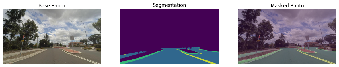
In this tutorial, a pre-trained road-segmentation-adas-0001 model from the Open Model Zoo is used. ADAS stands for Advanced Driver Assistance Services. The model recognizes four classes: background, road, curb and mark.

Table of contents:

• Imports

• Download model weights

• Select inference device

• Load the Model

• Load an Image

• Do Inference

• Prepare Data for Visualization

• Visualize data

Installation Instructions

This is a self-contained example that relies solely on its own code.

We recommend running the notebook in a virtual environment. You only need a Jupyter server to start. For details, please refer to Installation Guide.

# Install required packages
%pip install -q "openvino>=2023.1.0" opencv-python tqdm "matplotlib>=3.4"

Note: you may need to restart the kernel to use updated packages.

Imports

import cv2
import matplotlib.pyplot as plt
import numpy as np
import openvino as ov

# Fetch `notebook_utils` module
import requests

r = requests.get(
    url="https://raw.githubusercontent.com/openvinotoolkit/openvino_notebooks/latest/utils/notebook_utils.py",
)

open("notebook_utils.py", "w").write(r.text)

from notebook_utils import segmentation_map_to_image, download_file, device_widget

Download model weights

from pathlib import Path

base_model_dir = Path("./model").expanduser()

model_name = "road-segmentation-adas-0001"
model_xml_name = f"{model_name}.xml"
model_bin_name = f"{model_name}.bin"

model_xml_path = base_model_dir / model_xml_name

if not model_xml_path.exists():
    model_xml_url = (
        "https://storage.openvinotoolkit.org/repositories/open_model_zoo/2023.0/models_bin/1/road-segmentation-adas-0001/FP32/road-segmentation-adas-0001.xml"
    )
    model_bin_url = (
        "https://storage.openvinotoolkit.org/repositories/open_model_zoo/2023.0/models_bin/1/road-segmentation-adas-0001/FP32/road-segmentation-adas-0001.bin"
    )

    download_file(model_xml_url, model_xml_name, base_model_dir)
    download_file(model_bin_url, model_bin_name, base_model_dir)
else:
    print(f"{model_name} already downloaded to {base_model_dir}")

road-segmentation-adas-0001.xml:   0%|          | 0.00/389k [00:00<?, ?B/s]

road-segmentation-adas-0001.bin:   0%|          | 0.00/720k [00:00<?, ?B/s]

Select inference device

select device from dropdown list for running inference using OpenVINO

device = device_widget()
device

Dropdown(description='Device:', index=1, options=('CPU', 'AUTO'), value='AUTO')

Load the Model

core = ov.Core()

model = core.read_model(model=model_xml_path)
compiled_model = core.compile_model(model=model, device_name=device.value)

input_layer_ir = compiled_model.input(0)
output_layer_ir = compiled_model.output(0)

Load an Image

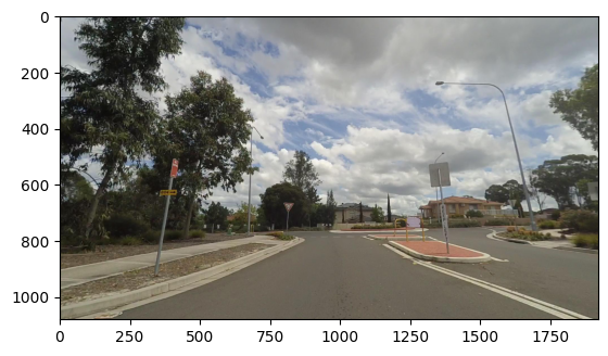
A sample image from the Mapillary Vistas dataset is provided.

# Download the image from the openvino_notebooks storage
image_filename = download_file(
    "https://storage.openvinotoolkit.org/repositories/openvino_notebooks/data/data/image/empty_road_mapillary.jpg",
    directory="data",
)

# The segmentation network expects images in BGR format.
image = cv2.imread(str(image_filename))

rgb_image = cv2.cvtColor(image, cv2.COLOR_BGR2RGB)
image_h, image_w, _ = image.shape

# N,C,H,W = batch size, number of channels, height, width.
N, C, H, W = input_layer_ir.shape

# OpenCV resize expects the destination size as (width, height).
resized_image = cv2.resize(image, (W, H))

# Reshape to the network input shape.
input_image = np.expand_dims(resized_image.transpose(2, 0, 1), 0)
plt.imshow(rgb_image)

empty_road_mapillary.jpg:   0%|          | 0.00/227k [00:00<?, ?B/s]

<matplotlib.image.AxesImage at 0x7f620b9afe50>

Do Inference

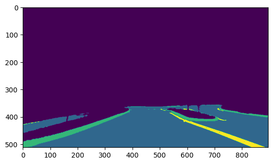
# Run the inference.
result = compiled_model([input_image])[output_layer_ir]

# Prepare data for visualization.
segmentation_mask = np.argmax(result, axis=1)
plt.imshow(segmentation_mask.transpose(1, 2, 0))

<matplotlib.image.AxesImage at 0x7f61bc2f8a00>

Prepare Data for Visualization

# Define colormap, each color represents a class.
colormap = np.array([[68, 1, 84], [48, 103, 141], [53, 183, 120], [199, 216, 52]])

# Define the transparency of the segmentation mask on the photo.
alpha = 0.3

# Use function from notebook_utils.py to transform mask to an RGB image.
mask = segmentation_map_to_image(segmentation_mask, colormap)
resized_mask = cv2.resize(mask, (image_w, image_h))

# Create an image with mask.
image_with_mask = cv2.addWeighted(resized_mask, alpha, rgb_image, 1 - alpha, 0)

Visualize data

# Define titles with images.
data = {"Base Photo": rgb_image, "Segmentation": mask, "Masked Photo": image_with_mask}

# Create a subplot to visualize images.
fig, axs = plt.subplots(1, len(data.items()), figsize=(15, 10))

# Fill the subplot.
for ax, (name, image) in zip(axs, data.items()):
    ax.axis("off")
    ax.set_title(name)
    ax.imshow(image)

# Display an image.
plt.show(fig)