Monocular Visual-Inertial Depth Estimation using OpenVINO™
This Jupyter notebook can be launched after a local installation only.
The overall methodology. Diagram taken from the VI-Depth repository.
A visual-inertial depth estimation pipeline that integrates monocular depth estimation and visual-inertial odometry to produce dense depth estimates with metric scale has been presented by the authors. The approach consists of three stages:
input processing, where RGB and inertial measurement unit (IMU) data feed into monocular depth estimation alongside visual-inertial odometry,
global scale and shift alignment, where monocular depth estimates are fitted to sparse depth from visual inertial odometry (VIO) in a least-squares manner and
learning-based dense scale alignment, where globally-aligned depth is locally realigned using a dense scale map regressed by the ScaleMapLearner (SML).
The images at the bottom in the diagram above illustrate a Visual Odometry with Inertial and Depth (VOID) sample being processed through our pipeline; from left to right: the input RGB, ground truth depth, sparse depth from VIO, globally-aligned depth, scale map scaffolding, dense scale map regressed by SML, final depth output.
An illustration of VOID samples being processed by the image pipeline.
Image taken from the VI-Depth repository.
We will be consulting the VI-Depth repository for the pre-processing, model transformations and basic utility code. A part of it has already been kept as it is in the utils directory. At the same time we will learn how to perform model conversion for converting a model in a different format to the standard OpenVINO™ IR model representation via another format.
Table of contents:
Imports
# Import sys beforehand to inform of Python version <= 3.7 not being supported
import sys

if sys.version_info.minor < 8:
    print('Python3.7 is not supported. Some features might not work as expected')

# Download the correct version of the PyTorch deep learning library associated with image models
# alongside the lightning module
%pip uninstall -q -y openvino-dev openvino openvino-nightly
%pip install -q --extra-index-url https://download.pytorch.org/whl/cpu "pytorch-lightning" "timm>=0.6.12" "openvino-nightly"
Note: you may need to restart the kernel to use updated packages.
DEPRECATION: pytorch-lightning 1.6.5 has a non-standard dependency specifier torch>=1.8.*. pip 24.1 will enforce this behaviour change. A possible replacement is to upgrade to a newer version of pytorch-lightning or contact the author to suggest that they release a version with a conforming dependency specifiers. Discussion can be found at https://github.com/pypa/pip/issues/12063
ERROR: pip's dependency resolver does not currently take into account all the packages that are installed. This behaviour is the source of the following dependency conflicts.
googleapis-common-protos 1.62.0 requires protobuf!=3.20.0,!=3.20.1,!=4.21.1,!=4.21.2,!=4.21.3,!=4.21.4,!=4.21.5,<5.0.0.dev0,>=3.19.5, but you have protobuf 3.20.1 which is incompatible.
onnx 1.15.0 requires protobuf>=3.20.2, but you have protobuf 3.20.1 which is incompatible.
paddlepaddle 2.6.0 requires protobuf>=3.20.2; platform_system != "Windows", but you have protobuf 3.20.1 which is incompatible.
tensorflow 2.12.0 requires protobuf!=4.21.0,!=4.21.1,!=4.21.2,!=4.21.3,!=4.21.4,!=4.21.5,<5.0.0dev,>=3.20.3, but you have protobuf 3.20.1 which is incompatible.
tensorflow-metadata 1.14.0 requires protobuf<4.21,>=3.20.3, but you have protobuf 3.20.1 which is incompatible.
Note: you may need to restart the kernel to use updated packages.
import matplotlib.pyplot as plt
import matplotlib.image as mpimg
import numpy as np
import openvino as ov
import torch
import torchvision
from pathlib import Path
from shutil import rmtree
from typing import Optional, Tuple

sys.path.append('../utils')
from notebook_utils import download_file

sys.path.append('vi_depth_utils')
import data_loader
import modules.midas.transforms as transforms
import modules.midas.utils as utils
from modules.estimator import LeastSquaresEstimator
from modules.interpolator import Interpolator2D
from modules.midas.midas_net_custom import MidasNet_small_videpth
# Ability to display images inline
%matplotlib inline
Loading models and checkpoints
The complete pipeline here requires only two models: one for depth estimation and a ScaleMapLearner model which is responsible for regressing a dense scale map. The table of models which has been given in the original VI-Depth repo has been presented as it is for the users to download from. VOID is the name of the original dataset from on which these models have been trained. The numbers after the word VOID represent the checkpoint in the model obtained after training samples for sparse dense maps corresponding to \(150\), \(500\) and \(1500\) levels in the density map. Just right-click on any of the highlighted links and click on “Copy link address”. We shall use this link in the next cell to download the ScaleMapLearner model. Interestingly, the ScaleMapLearner decides the depth prediction model as you will see.
Depth Predictor |
SML on VOID 150 |
SML on VOID 500 |
SML on VOID 1500 |
|---|---|---|---|
DPT-BEiT-Large |
|||
DPT-SwinV2-Large |
|||
DPT-Large |
|||
DPT-Hybrid |
|||
DPT-SwinV2-Tiny |
|||
DPT-LeViT |
|||
MiDaS-small |
*Also available with pre-training on TartanAir: model
# Base directory in which models would be stored as a pathlib.Path variable
MODEL_DIR = Path('model')

# Mapping between depth predictors and the corresponding scale map learners
PREDICTOR_MODEL_MAP = {'dpt_beit_large_512': 'DPT_BEiT_L_512',
                       'dpt_swin2_large_384': 'DPT_SwinV2_L_384',
                       'dpt_large': 'DPT_Large',
                       'dpt_hybrid': 'DPT_Hybrid',
                       'dpt_swin2_tiny_256': 'DPT_SwinV2_T_256',
                       'dpt_levit_224': 'DPT_LeViT_224',
                       'midas_small': 'MiDaS_small'}
# Create the model directory adjacent to the notebook and suppress errors if the directory already exists
MODEL_DIR.mkdir(exist_ok=True)

# Here we will be downloading the SML model corresponding to the MiDaS-small depth predictor for
# the checkpoint captured after training on 1500 points of the density level. Suppress errors if the file already exists
download_file('https://github.com/isl-org/VI-Depth/releases/download/v1/sml_model.dpredictor.midas_small.nsamples.1500.ckpt', directory=MODEL_DIR, silent=True)

# Take a note of the samples. It would be of major use later on
NSAMPLES = 1500
model/sml_model.dpredictor.midas_small.nsamples.1500.ckpt: 0%| | 0.00/208M [00:00<?, ?B/s]
# Set the same model directory for downloading the depth predictor model which is available on
# PyTorch hub
torch.hub.set_dir(str(MODEL_DIR))


# A utility function for utilising the mapping between depth predictors and
# scale map learners so as to download the former
def get_model_for_predictor(depth_predictor: str, remote_repo: str = 'intel-isl/MiDaS') -> str:
    """
    Download a model from the pre-validated 'isl-org/MiDaS:2.1' set of releases on the GitHub repo
    while simultaneously trusting the repo permanently

    :param: depth_predictor: Any depth estimation model amongst the ones given at https://github.com/isl-org/VI-Depth#setup
    :param: remote_repo: The remote GitHub repo from where the models will be downloaded
    :returns: A PyTorch model callable
    """

    # Workaround for avoiding rate limit errors
    torch.hub._validate_not_a_forked_repo = lambda a, b, c: True

    return torch.hub.load(remote_repo, PREDICTOR_MODEL_MAP[depth_predictor], skip_validation=True, trust_repo=True)
# Execute the above function so as to download the MiDaS-small model
# and get the output of the model callable in return
depth_model = get_model_for_predictor('midas_small')
Downloading: "https://github.com/intel-isl/MiDaS/zipball/master" to model/master.zip
Loading weights: None
/opt/home/k8sworker/ci-ai/cibuilds/ov-notebook/OVNotebookOps-609/.workspace/scm/ov-notebook/.venv/lib/python3.8/site-packages/torch/hub.py:294: UserWarning: You are about to download and run code from an untrusted repository. In a future release, this won't be allowed. To add the repository to your trusted list, change the command to {calling_fn}(..., trust_repo=False) and a command prompt will appear asking for an explicit confirmation of trust, or load(..., trust_repo=True), which will assume that the prompt is to be answered with 'yes'. You can also use load(..., trust_repo='check') which will only prompt for confirmation if the repo is not already trusted. This will eventually be the default behaviour
  warnings.warn(
Downloading: "https://github.com/rwightman/gen-efficientnet-pytorch/zipball/master" to model/master.zip
Downloading: "https://github.com/rwightman/pytorch-image-models/releases/download/v0.1-weights/tf_efficientnet_lite3-b733e338.pth" to model/checkpoints/tf_efficientnet_lite3-b733e338.pth
Downloading: "https://github.com/isl-org/MiDaS/releases/download/v2_1/midas_v21_small_256.pt" to model/checkpoints/midas_v21_small_256.pt
0%| | 0.00/81.8M [00:00<?, ?B/s]
0%| | 320k/81.8M [00:00<00:27, 3.15MB/s]
1%| | 720k/81.8M [00:00<00:23, 3.68MB/s]
1%|▏ | 1.08M/81.8M [00:00<00:22, 3.78MB/s]
2%|▏ | 1.47M/81.8M [00:00<00:21, 3.88MB/s]
2%|▏ | 1.86M/81.8M [00:00<00:21, 3.83MB/s]
3%|▎ | 2.27M/81.8M [00:00<00:21, 3.95MB/s]
3%|▎ | 2.67M/81.8M [00:00<00:20, 4.05MB/s]
4%|▎ | 3.06M/81.8M [00:00<00:23, 3.55MB/s]
4%|▍ | 3.44M/81.8M [00:00<00:23, 3.53MB/s]
5%|▍ | 3.86M/81.8M [00:01<00:21, 3.76MB/s]
5%|▌ | 4.27M/81.8M [00:01<00:21, 3.84MB/s]
6%|▌ | 4.66M/81.8M [00:01<00:20, 3.90MB/s]
6%|▌ | 5.05M/81.8M [00:01<00:21, 3.81MB/s]
7%|▋ | 5.45M/81.8M [00:01<00:20, 3.94MB/s]
7%|▋ | 5.86M/81.8M [00:01<00:19, 4.03MB/s]
8%|▊ | 6.25M/81.8M [00:01<00:19, 4.01MB/s]
8%|▊ | 6.64M/81.8M [00:01<00:19, 4.02MB/s]
9%|▊ | 7.03M/81.8M [00:01<00:20, 3.89MB/s]
9%|▉ | 7.43M/81.8M [00:02<00:19, 3.97MB/s]
10%|▉ | 7.84M/81.8M [00:02<00:19, 4.07MB/s]
10%|█ | 8.23M/81.8M [00:02<00:19, 4.03MB/s]
11%|█ | 8.64M/81.8M [00:02<00:18, 4.05MB/s]
11%|█ | 9.03M/81.8M [00:02<00:19, 3.92MB/s]
12%|█▏ | 9.45M/81.8M [00:02<00:18, 4.06MB/s]
12%|█▏ | 9.84M/81.8M [00:02<00:18, 4.01MB/s]
13%|█▎ | 10.2M/81.8M [00:02<00:18, 4.05MB/s]
13%|█▎ | 10.6M/81.8M [00:02<00:19, 3.92MB/s]
13%|█▎ | 11.0M/81.8M [00:02<00:19, 3.86MB/s]
14%|█▍ | 11.4M/81.8M [00:03<00:18, 3.97MB/s]
14%|█▍ | 11.8M/81.8M [00:03<00:18, 4.04MB/s]
15%|█▍ | 12.2M/81.8M [00:03<00:17, 4.10MB/s]
15%|█▌ | 12.6M/81.8M [00:03<00:18, 3.99MB/s]
16%|█▌ | 13.0M/81.8M [00:03<00:18, 3.91MB/s]
16%|█▋ | 13.4M/81.8M [00:03<00:17, 4.01MB/s]
17%|█▋ | 13.8M/81.8M [00:03<00:17, 4.07MB/s]
17%|█▋ | 14.2M/81.8M [00:03<00:17, 4.11MB/s]
18%|█▊ | 14.6M/81.8M [00:03<00:18, 3.91MB/s]
18%|█▊ | 15.0M/81.8M [00:04<00:17, 3.98MB/s]
19%|█▉ | 15.5M/81.8M [00:04<00:17, 4.09MB/s]
19%|█▉ | 15.9M/81.8M [00:04<00:17, 3.91MB/s]
20%|█▉ | 16.2M/81.8M [00:04<00:17, 3.95MB/s]
20%|██ | 16.7M/81.8M [00:04<00:16, 4.03MB/s]
21%|██ | 17.1M/81.8M [00:04<00:16, 4.08MB/s]
21%|██▏ | 17.5M/81.8M [00:04<00:16, 4.02MB/s]
22%|██▏ | 17.9M/81.8M [00:04<00:17, 3.93MB/s]
22%|██▏ | 18.2M/81.8M [00:04<00:16, 3.96MB/s]
23%|██▎ | 18.7M/81.8M [00:04<00:16, 4.10MB/s]
23%|██▎ | 19.1M/81.8M [00:05<00:16, 4.04MB/s]
24%|██▍ | 19.5M/81.8M [00:05<00:16, 3.95MB/s]
24%|██▍ | 19.9M/81.8M [00:05<00:16, 3.97MB/s]
25%|██▍ | 20.2M/81.8M [00:05<00:16, 4.00MB/s]
25%|██▌ | 20.7M/81.8M [00:05<00:15, 4.07MB/s]
26%|██▌ | 21.1M/81.8M [00:05<00:16, 3.98MB/s]
26%|██▌ | 21.5M/81.8M [00:05<00:15, 3.97MB/s]
27%|██▋ | 21.9M/81.8M [00:05<00:15, 4.00MB/s]
27%|██▋ | 22.2M/81.8M [00:05<00:15, 4.02MB/s]
28%|██▊ | 22.7M/81.8M [00:06<00:15, 4.03MB/s]
28%|██▊ | 23.1M/81.8M [00:06<00:15, 3.99MB/s]
29%|██▊ | 23.5M/81.8M [00:06<00:15, 4.00MB/s]
29%|██▉ | 23.9M/81.8M [00:06<00:15, 4.04MB/s]
30%|██▉ | 24.3M/81.8M [00:06<00:14, 4.03MB/s]
30%|███ | 24.7M/81.8M [00:06<00:14, 4.04MB/s]
31%|███ | 25.1M/81.8M [00:06<00:14, 3.98MB/s]
31%|███ | 25.5M/81.8M [00:06<00:14, 3.99MB/s]
32%|███▏ | 25.9M/81.8M [00:06<00:14, 4.04MB/s]
32%|███▏ | 26.2M/81.8M [00:06<00:14, 4.06MB/s]
33%|███▎ | 26.6M/81.8M [00:07<00:14, 4.04MB/s]
33%|███▎ | 27.0M/81.8M [00:07<00:14, 4.04MB/s]
34%|███▎ | 27.4M/81.8M [00:07<00:14, 3.96MB/s]
34%|███▍ | 27.8M/81.8M [00:07<00:14, 3.96MB/s]
35%|███▍ | 28.2M/81.8M [00:07<00:13, 4.03MB/s]
35%|███▍ | 28.6M/81.8M [00:07<00:13, 4.03MB/s]
35%|███▌ | 29.0M/81.8M [00:07<00:13, 4.04MB/s]
36%|███▌ | 29.4M/81.8M [00:07<00:13, 4.04MB/s]
36%|███▋ | 29.8M/81.8M [00:07<00:13, 3.97MB/s]
37%|███▋ | 30.2M/81.8M [00:07<00:13, 3.98MB/s]
37%|███▋ | 30.6M/81.8M [00:08<00:13, 3.99MB/s]
38%|███▊ | 31.0M/81.8M [00:08<00:13, 4.02MB/s]
38%|███▊ | 31.4M/81.8M [00:08<00:13, 4.04MB/s]
39%|███▉ | 31.8M/81.8M [00:08<00:12, 4.04MB/s]
39%|███▉ | 32.1M/81.8M [00:08<00:13, 3.97MB/s]
40%|███▉ | 32.5M/81.8M [00:08<00:12, 3.99MB/s]
40%|████ | 32.9M/81.8M [00:08<00:12, 3.99MB/s]
41%|████ | 33.3M/81.8M [00:08<00:12, 4.06MB/s]
41%|████ | 33.7M/81.8M [00:08<00:12, 4.06MB/s]
42%|████▏ | 34.1M/81.8M [00:09<00:12, 3.99MB/s]
42%|████▏ | 34.5M/81.8M [00:09<00:12, 4.00MB/s]
43%|████▎ | 34.9M/81.8M [00:09<00:12, 3.99MB/s]
43%|████▎ | 35.3M/81.8M [00:09<00:12, 4.01MB/s]
44%|████▎ | 35.7M/81.8M [00:09<00:11, 4.07MB/s]
44%|████▍ | 36.1M/81.8M [00:09<00:11, 4.06MB/s]
45%|████▍ | 36.5M/81.8M [00:09<00:11, 4.05MB/s]
45%|████▌ | 36.9M/81.8M [00:09<00:11, 3.94MB/s]
46%|████▌ | 37.3M/81.8M [00:09<00:11, 3.98MB/s]
46%|████▌ | 37.7M/81.8M [00:09<00:11, 4.00MB/s]
47%|████▋ | 38.1M/81.8M [00:10<00:11, 4.07MB/s]
47%|████▋ | 38.5M/81.8M [00:10<00:11, 4.05MB/s]
47%|████▋ | 38.8M/81.8M [00:10<00:11, 4.04MB/s]
48%|████▊ | 39.2M/81.8M [00:10<00:11, 3.98MB/s]
48%|████▊ | 39.6M/81.8M [00:10<00:11, 3.98MB/s]
49%|████▉ | 40.0M/81.8M [00:10<00:11, 3.97MB/s]
49%|████▉ | 40.4M/81.8M [00:10<00:10, 4.03MB/s]
50%|████▉ | 40.8M/81.8M [00:10<00:10, 4.06MB/s]
50%|█████ | 41.2M/81.8M [00:10<00:10, 4.03MB/s]
51%|█████ | 41.6M/81.8M [00:10<00:10, 3.96MB/s]
51%|█████▏ | 42.0M/81.8M [00:11<00:10, 3.97MB/s]
52%|█████▏ | 42.4M/81.8M [00:11<00:10, 4.00MB/s]
52%|█████▏ | 42.8M/81.8M [00:11<00:10, 4.06MB/s]
53%|█████▎ | 43.2M/81.8M [00:11<00:09, 4.05MB/s]
53%|█████▎ | 43.6M/81.8M [00:11<00:09, 4.05MB/s]
54%|█████▎ | 44.0M/81.8M [00:11<00:09, 3.99MB/s]
54%|█████▍ | 44.3M/81.8M [00:11<00:09, 3.94MB/s]
55%|█████▍ | 44.8M/81.8M [00:11<00:09, 4.03MB/s]
55%|█████▌ | 45.2M/81.8M [00:11<00:09, 4.08MB/s]
56%|█████▌ | 45.5M/81.8M [00:11<00:09, 4.03MB/s]
56%|█████▌ | 45.9M/81.8M [00:12<00:09, 3.99MB/s]
57%|█████▋ | 46.3M/81.8M [00:12<00:09, 3.98MB/s]
57%|█████▋ | 46.7M/81.8M [00:12<00:09, 3.97MB/s]
58%|█████▊ | 47.1M/81.8M [00:12<00:08, 4.05MB/s]
58%|█████▊ | 47.5M/81.8M [00:12<00:08, 4.04MB/s]
59%|█████▊ | 47.9M/81.8M [00:12<00:08, 4.00MB/s]
59%|█████▉ | 48.3M/81.8M [00:12<00:08, 3.98MB/s]
60%|█████▉ | 48.7M/81.8M [00:12<00:08, 3.98MB/s]
60%|██████ | 49.1M/81.8M [00:12<00:08, 4.08MB/s]
61%|██████ | 49.5M/81.8M [00:13<00:08, 4.03MB/s]
61%|██████ | 49.9M/81.8M [00:13<00:08, 4.03MB/s]
61%|██████▏ | 50.3M/81.8M [00:13<00:08, 3.98MB/s]
62%|██████▏ | 50.7M/81.8M [00:13<00:08, 3.91MB/s]
62%|██████▏ | 51.1M/81.8M [00:13<00:08, 4.02MB/s]
63%|██████▎ | 51.5M/81.8M [00:13<00:07, 4.08MB/s]
63%|██████▎ | 51.9M/81.8M [00:13<00:07, 4.03MB/s]
64%|██████▍ | 52.3M/81.8M [00:13<00:07, 3.91MB/s]
64%|██████▍ | 52.7M/81.8M [00:13<00:07, 4.01MB/s]
65%|██████▍ | 53.1M/81.8M [00:13<00:07, 4.04MB/s]
65%|██████▌ | 53.5M/81.8M [00:14<00:07, 4.05MB/s]
66%|██████▌ | 53.9M/81.8M [00:14<00:07, 4.02MB/s]
66%|██████▋ | 54.3M/81.8M [00:14<00:07, 3.93MB/s]
67%|██████▋ | 54.7M/81.8M [00:14<00:07, 4.01MB/s]
67%|██████▋ | 55.1M/81.8M [00:14<00:06, 4.02MB/s]
68%|██████▊ | 55.5M/81.8M [00:14<00:06, 4.08MB/s]
68%|██████▊ | 55.9M/81.8M [00:14<00:06, 4.04MB/s]
69%|██████▉ | 56.3M/81.8M [00:14<00:06, 3.93MB/s]
69%|██████▉ | 56.7M/81.8M [00:14<00:06, 3.98MB/s]
70%|██████▉ | 57.1M/81.8M [00:14<00:06, 4.04MB/s]
70%|███████ | 57.5M/81.8M [00:15<00:06, 4.04MB/s]
71%|███████ | 57.9M/81.8M [00:15<00:06, 4.06MB/s]
71%|███████ | 58.3M/81.8M [00:15<00:06, 3.94MB/s]
72%|███████▏ | 58.7M/81.8M [00:15<00:06, 3.98MB/s]
72%|███████▏ | 59.0M/81.8M [00:15<00:05, 4.01MB/s]
73%|███████▎ | 59.4M/81.8M [00:15<00:06, 3.76MB/s]
73%|███████▎ | 59.9M/81.8M [00:15<00:05, 3.97MB/s]
74%|███████▎ | 60.3M/81.8M [00:15<00:05, 4.09MB/s]
74%|███████▍ | 60.7M/81.8M [00:15<00:05, 3.84MB/s]
75%|███████▍ | 61.1M/81.8M [00:16<00:05, 3.98MB/s]
75%|███████▌ | 61.5M/81.8M [00:16<00:05, 4.09MB/s]
76%|███████▌ | 61.9M/81.8M [00:16<00:05, 3.88MB/s]
76%|███████▌ | 62.3M/81.8M [00:16<00:05, 3.90MB/s]
77%|███████▋ | 62.7M/81.8M [00:16<00:04, 4.09MB/s]
77%|███████▋ | 63.1M/81.8M [00:16<00:05, 3.89MB/s]
78%|███████▊ | 63.5M/81.8M [00:16<00:04, 3.93MB/s]
78%|███████▊ | 63.9M/81.8M [00:16<00:04, 3.98MB/s]
79%|███████▊ | 64.3M/81.8M [00:16<00:04, 4.10MB/s]
79%|███████▉ | 64.8M/81.8M [00:17<00:04, 3.95MB/s]
80%|███████▉ | 65.2M/81.8M [00:17<00:04, 3.97MB/s]
80%|████████ | 65.6M/81.8M [00:17<00:04, 4.05MB/s]
81%|████████ | 66.0M/81.8M [00:17<00:03, 4.18MB/s]
81%|████████ | 66.4M/81.8M [00:17<00:04, 3.93MB/s]
82%|████████▏ | 66.8M/81.8M [00:17<00:03, 4.00MB/s]
82%|████████▏ | 67.2M/81.8M [00:17<00:03, 4.15MB/s]
83%|████████▎ | 67.6M/81.8M [00:17<00:03, 3.93MB/s]
83%|████████▎ | 68.0M/81.8M [00:17<00:03, 3.93MB/s]
84%|████████▎ | 68.4M/81.8M [00:17<00:03, 3.95MB/s]
84%|████████▍ | 68.8M/81.8M [00:18<00:04, 3.23MB/s]
85%|████████▍ | 69.2M/81.8M [00:18<00:03, 3.47MB/s]
85%|████████▌ | 69.6M/81.8M [00:18<00:03, 3.44MB/s]
86%|████████▌ | 70.0M/81.8M [00:18<00:03, 3.65MB/s]
86%|████████▌ | 70.4M/81.8M [00:18<00:03, 3.81MB/s]
87%|████████▋ | 70.8M/81.8M [00:18<00:03, 3.74MB/s]
87%|████████▋ | 71.2M/81.8M [00:18<00:02, 3.84MB/s]
88%|████████▊ | 71.7M/81.8M [00:18<00:02, 4.00MB/s]
88%|████████▊ | 72.1M/81.8M [00:19<00:02, 4.11MB/s]
89%|████████▊ | 72.5M/81.8M [00:19<00:02, 3.87MB/s]
89%|████████▉ | 72.9M/81.8M [00:19<00:02, 3.99MB/s]
90%|████████▉ | 73.3M/81.8M [00:19<00:02, 4.07MB/s]
90%|█████████ | 73.7M/81.8M [00:19<00:02, 3.88MB/s]
91%|█████████ | 74.1M/81.8M [00:19<00:02, 3.93MB/s]
91%|█████████ | 74.5M/81.8M [00:19<00:01, 4.02MB/s]
92%|█████████▏| 74.9M/81.8M [00:19<00:01, 4.13MB/s]
92%|█████████▏| 75.3M/81.8M [00:19<00:01, 3.93MB/s]
93%|█████████▎| 75.7M/81.8M [00:19<00:01, 3.93MB/s]
93%|█████████▎| 76.1M/81.8M [00:20<00:01, 3.98MB/s]
94%|█████████▎| 76.5M/81.8M [00:20<00:01, 4.10MB/s]
94%|█████████▍| 76.9M/81.8M [00:20<00:01, 4.15MB/s]
95%|█████████▍| 77.3M/81.8M [00:20<00:01, 3.94MB/s]
95%|█████████▌| 77.7M/81.8M [00:20<00:01, 3.94MB/s]
96%|█████████▌| 78.1M/81.8M [00:20<00:00, 4.03MB/s]
96%|█████████▌| 78.5M/81.8M [00:20<00:00, 4.14MB/s]
97%|█████████▋| 78.9M/81.8M [00:20<00:00, 3.93MB/s]
97%|█████████▋| 79.3M/81.8M [00:20<00:00, 3.94MB/s]
97%|█████████▋| 79.7M/81.8M [00:21<00:00, 3.98MB/s]
98%|█████████▊| 80.1M/81.8M [00:21<00:00, 4.11MB/s]
98%|█████████▊| 80.5M/81.8M [00:21<00:00, 3.93MB/s]
99%|█████████▉| 80.9M/81.8M [00:21<00:00, 3.97MB/s]
99%|█████████▉| 81.3M/81.8M [00:21<00:00, 4.00MB/s]
100%|█████████▉| 81.7M/81.8M [00:21<00:00, 4.07MB/s]
100%|██████████| 81.8M/81.8M [00:21<00:00, 3.98MB/s]
Cleaning up the model directory
From the verbose of the previous step it is obvious that torch.hub.load downloads a lot of unnecessary files. We shall move remove the unnecessary directories and files which were created during the download process.
# Remove unnecessary directories and files and suppress errors(if any)
rmtree(path=str(MODEL_DIR / 'intel-isl_MiDaS_master'), ignore_errors=True)
rmtree(path=str(MODEL_DIR / 'rwightman_gen-efficientnet-pytorch_master'), ignore_errors=True)
rmtree(path=str(MODEL_DIR / 'checkpoints'), ignore_errors=True)

# Check for the existence of the trusted list file and then remove
list_file = Path(MODEL_DIR / 'trusted_list')
if list_file.is_file():
    list_file.unlink()
Transformation of models
Each of the models need an appropriate transformation which can be
invoked by the get_model_transforms function. It needs only the
depth_predictor parameter and NSAMPLES defined above to work.
The reason being that the ScaleMapLearner and the depth estimation
model are always in direct correspondence with each other.
# Define important custom types
type_transform_compose = torchvision.transforms.transforms.Compose
type_compiled_model = ov.CompiledModel
def get_model_transforms(depth_predictor: str, nsamples: int) -> Tuple[type_transform_compose, type_transform_compose]:
    """
    Construct the transformation of the depth prediction model and the
    associated ScaleMapLearner model

    :param: depth_predictor: Any depth estimation model amongst the ones given at https://github.com/isl-org/VI-Depth#setup
    :param: nsamples: The no. of density levels for the depth map
    :returns: The transformed models as the resut of torchvision.transforms.Compose operations
    """
    model_transforms = transforms.get_transforms(depth_predictor, "void", str(nsamples))
    return model_transforms['depth_model'], model_transforms['sml_model']
# Obtain transforms of both the models here
depth_model_transform, scale_map_learner_transform = get_model_transforms(depth_predictor='midas_small',
                                                                          nsamples=NSAMPLES)
Dummy input creation
Dummy inputs help during conversion. Although ov.convert_model
accepts any dummy input for a single pass through the model and thereby
enabling model conversion, the pre-processing required for the actual
inputs later at inference using compiled models would be substantial. So
we have decided that even dummy inputs should go through the proper
transformation process so that the reader gets the idea of a
transformed image being compiled by a transformed model.
Also note down the width and height of the image which would be used multiple times later. Do note that this is constant throughout the dataset
IMAGE_H, IMAGE_W = 480, 640

# Although you can always verify the same by uncommenting and running
# the following lines
# img = cv2.imread('data/image/dummy_img.png')
# print(img.shape)
# Base directory in which data would be stored as a pathlib.Path variable
DATA_DIR = Path('data')

# Create the data directory tree adjacent to the notebook and suppress errors if the directory already exists
# Create a directory each for the images and their corresponding depth maps
DATA_DIR.mkdir(exist_ok=True)
Path(DATA_DIR / 'image').mkdir(exist_ok=True)
Path(DATA_DIR / 'sparse_depth').mkdir(exist_ok=True)

# Download the dummy image and its depth scale (take a note of the image hashes for possible later use)
# On the fly download is being done to avoid unnecessary memory/data load during testing and
# creation of PRs
download_file('https://user-images.githubusercontent.com/22426058/254174385-161b9f0e-5991-4308-ba89-d81bc02bcb7c.png', filename='dummy_img.png', directory=Path(DATA_DIR / 'image'), silent=True)
download_file('https://user-images.githubusercontent.com/22426058/254174398-8c71c59f-0adf-43c6-ad13-c04431e02349.png', filename='dummy_depth.png', directory=Path(DATA_DIR / 'sparse_depth'), silent=True)

# Load the dummy image and its depth scale
dummy_input = data_loader.load_input_image('data/image/dummy_img.png')
dummy_depth = data_loader.load_sparse_depth('data/sparse_depth/dummy_depth.png')
data/image/dummy_img.png: 0%| | 0.00/328k [00:00<?, ?B/s]
data/sparse_depth/dummy_depth.png: 0%| | 0.00/765 [00:00<?, ?B/s]
def transform_image_for_depth(input_image: np.ndarray, depth_model_transform: np.ndarray, device: torch.device = 'cpu') -> torch.Tensor:
    """
    Transform the input_image for processing by a PyTorch depth estimation model

    :param: input_image: The input image obtained as a result of data_loader.load_input_image
    :param: depth_model_transform: The transformed depth model
    :param: device: The device on which the image would be allocated
    :returns: The transformed image suitable to be used as an input to the depth estimation model
    """
    input_height, input_width = np.shape(input_image)[:2]

    sample = {'image' : input_image}
    sample = depth_model_transform(sample)
    im = sample['image'].to(device)
    return im.unsqueeze(0)
# Transform the dummy input image for the depth model
transformed_dummy_image = transform_image_for_depth(input_image=dummy_input, depth_model_transform=depth_model_transform)
Conversion of depth model to OpenVINO IR format
Starting from 2023.0.0 release, OpenVINO supports PyTorch model via conversion to OpenVINO Intermediate Representation format (IR). To have a depth estimation model in the OpenVINO™ IR format and then compile it, we shall follow the following steps:
Use the
depth_modelcallable to our advantage from the Loading models and checkpoints stage.Convert PyTorch model to OpenVINO model using OpenVINO Model conversion API and the transformed dummy input created earlier.
Use the
ov.save_modelfunction from OpenVINO to serialize OpenVINO.xmland.binfiles for next compilation skipping conversion step Alternatively serialization procedure may be avoided and compiled model may be obtained by directly using OpenVINO’scompile_modelfunction.
# Evaluate the model to switch some operations from training mode to inference.
depth_model.eval()


# Check PyTorch model work with dummy input
_ = depth_model(transformed_dummy_image)

# convert model to OpenVINO IR
ov_model = ov.convert_model(depth_model, example_input=(transformed_dummy_image, ))

# save model for next usage
ov.save_model(ov_model, 'depth_model.xml')
select device from dropdown list for running inference using OpenVINO
import ipywidgets as widgets

core = ov.Core()

device = widgets.Dropdown(
    options=core.available_devices + ["AUTO"],
    value='AUTO',
    description='Device:',
    disabled=False,
)

device
Dropdown(description='Device:', index=1, options=('CPU', 'AUTO'), value='AUTO')
Now we can go ahead and compile our depth model.
# Initialize OpenVINO Runtime.
compiled_depth_model = core.compile_model(model=ov_model, device_name=device.value)
def run_depth_model(input_image_h: int, input_image_w: int,
                    transformed_image: torch.Tensor, compiled_depth_model: type_compiled_model) -> np.ndarray:

    """
    Run the compiled_depth_model on the transformed_image of dimensions
    input_image_w x input_image_h

    :param: input_image_h: The height of the input image
    :param: input_image_w: The width of the input image
    :param: transformed_image: The transformed image suitable to be used as an input to the depth estimation model
    :returns:
             depth_pred: The depth prediction on the image as an np.ndarray type

    """

    # Obtain the last output layer separately
    output_layer_depth_model = compiled_depth_model.output(0)

    with torch.no_grad():
        # Perform computation like a standard OpenVINO compiled model
        depth_pred = torch.from_numpy(compiled_depth_model([transformed_image])[output_layer_depth_model])
        depth_pred = (
            torch.nn.functional.interpolate(
                depth_pred.unsqueeze(1),
                size=(input_image_h, input_image_w),
                mode='bicubic',
                align_corners=False,
            )
            .squeeze()
            .cpu()
            .numpy()
        )

    return depth_pred
# Run the compiled depth model using the dummy input
# It will be used to compute the metrics associated with the ScaleMapLearner model
# and hence obtain a compiled version of the same later
depth_pred_dummy = run_depth_model(input_image_h=IMAGE_H, input_image_w=IMAGE_W,
                                   transformed_image=transformed_dummy_image, compiled_depth_model=compiled_depth_model)
Computation of these parameters required the depth estimation model output from the previous step. These are the regression based parameters the ScaleMapLearner model deals with. An utility function for the purpose has already been created.
def compute_global_scale_and_shift(input_sparse_depth: np.ndarray, validity_map: Optional[np.ndarray],
                                   depth_pred: np.ndarray,
                                   min_pred: float = 0.1, max_pred: float = 8.0,
                                   min_depth: float = 0.2, max_depth: float = 5.0) -> Tuple[np.ndarray, np.ndarray]:

    """
    Compute the global scale and shift alignment required for SML model to work on
    with the input_sparse_depth map being provided and the depth estimation output depth_pred
    being provided with an optional validity_map

    :param: input_sparse_depth: The depth map of the input image
    :param: validity_map: An optional depth map associated with the original input image
    :param: depth_pred: The depth estimate obtained after running the depth model on the input image
    :param: min_pred: Lower bound for predicted depth values
    :param: max_pred: Upper bound for predicted depth values
    :param: min_depth: Min valid depth when evaluating
    :param: max_depth: Max valid depth when evaluating
    :returns:
             int_depth: The depth estimate for the SML regression model
             int_scales: The scale to be used for the SML regression model

    """

    input_sparse_depth_valid = (input_sparse_depth < max_depth) * (input_sparse_depth > min_depth)
    if validity_map is not None:
        input_sparse_depth_valid *= validity_map.astype(np.bool)

    input_sparse_depth_valid = input_sparse_depth_valid.astype(bool)
    input_sparse_depth[~input_sparse_depth_valid] = np.inf  # set invalid depth
    input_sparse_depth = 1.0 / input_sparse_depth

    # global scale and shift alignment
    GlobalAlignment = LeastSquaresEstimator(
        estimate=depth_pred,
        target=input_sparse_depth,
        valid=input_sparse_depth_valid
    )
    GlobalAlignment.compute_scale_and_shift()
    GlobalAlignment.apply_scale_and_shift()
    GlobalAlignment.clamp_min_max(clamp_min=min_pred, clamp_max=max_pred)
    int_depth = GlobalAlignment.output.astype(np.float32)

    # interpolation of scale map
    assert (np.sum(input_sparse_depth_valid) >= 3), 'not enough valid sparse points'
    ScaleMapInterpolator = Interpolator2D(
        pred_inv=int_depth,
        sparse_depth_inv=input_sparse_depth,
        valid=input_sparse_depth_valid,
    )
    ScaleMapInterpolator.generate_interpolated_scale_map(
        interpolate_method='linear',
        fill_corners=False
    )

    int_scales = ScaleMapInterpolator.interpolated_scale_map.astype(np.float32)
    int_scales = utils.normalize_unit_range(int_scales)

    return int_depth, int_scales
# Call the function on the dummy depth map we loaded in the dummy_depth variable
# with all default settings and store in appropriate variables
d_depth, d_scales = compute_global_scale_and_shift(input_sparse_depth=dummy_depth, validity_map=None, depth_pred=depth_pred_dummy)
def transform_image_for_depth_scale(input_image: np.ndarray, scale_map_learner_transform: type_transform_compose,
                                    int_depth: np.ndarray, int_scales: np.ndarray,
                                    device: torch.device = 'cpu') -> Tuple[torch.Tensor, torch.Tensor]:
    """
    Transform the input_image for processing by a PyTorch SML model

    :param: input_image: The input image obtained as a result of data_loader.load_input_image
    :param: scale_map_learner_transform: The transformed SML model
    :param: int_depth: The depth estimate for the SML regression model
    :param: int_scales: he scale to be used for the SML regression model
    :param: device: The device on which the image would be allocated
    :returns: The transformed tensor inputs suitable to be used with an SML model
    """

    sample = {'image' : input_image, 'int_depth' : int_depth, 'int_scales' : int_scales, 'int_depth_no_tf' : int_depth}
    sample = scale_map_learner_transform(sample)
    x = torch.cat([sample['int_depth'], sample['int_scales']], 0)
    x = x.to(device)
    d = sample['int_depth_no_tf'].to(device)

    return x.unsqueeze(0), d.unsqueeze(0)
# Transform the dummy input image for the ScaleMapLearner model
# Note that this will lead to a tuple as an output. Both the elements
# which is fed to ScaleMapLearner during the conversion process to onxx
transformed_dummy_image_scale = transform_image_for_depth_scale(input_image=dummy_input,
                                                                scale_map_learner_transform=scale_map_learner_transform,
                                                                int_depth=d_depth, int_scales=d_scales)
Conversion of Scale Map Learner model to OpenVINO IR format
The OpenVINO™ toolkit provides direct method of converting PyTorch models to the intermediate representation format. To have the associated ScaleMapLearner in the OpenVINO™ IR format and then compile it, we shall follow the following steps:
Load the model in memory via instantiating the
modules.midas.midas_net_custom.MidasNet_small_videpthclass and passing the downloaded checkpoint earlier as an argument.Convert PyTorch model to OpenVINO model using OpenVINO Model conversion API and the transformed dummy input created earlier.
Use the
ov.save_modelfunction from OpenVINO to serialize OpenVINO.xmland.binfiles for next compilation skipping conversion step Alternatively serialization procedure may be avoided and compiled model may be obtained by directly using OpenVINO’scompile_modelfunction.
If the name of the .ckpt file is too much to handle, here is the
common format of all checkpoint files from the model releases.
sml_model.dpredictor.<DEPTH_PREDICTOR>.nsamples.<NSAMPLES>.ckpt
Replace <DEPTH_PREDICTOR> and <NSAMPLES> with the depth estimation model name and the no. of levels of depth density the SML model has been trained on
E.g. sml_model.dpredictor.dpt_hybrid.nsamples.500.ckpt will be the file name corresponding to the SML model based on the dpt_hybrid depth predictor and has been trained on 500 points of the density level on the depth map
# Run with the same min_pred and max_pred arguments which were used to compute
# global scale and shift alignment
scale_map_learner = MidasNet_small_videpth(path=str(MODEL_DIR / 'sml_model.dpredictor.midas_small.nsamples.1500.ckpt'),
                                           min_pred=0.1, max_pred=8.0)
Loading weights: model/sml_model.dpredictor.midas_small.nsamples.1500.ckpt
Downloading: "https://github.com/rwightman/gen-efficientnet-pytorch/zipball/master" to model/master.zip
2024-02-10 00:24:12.163962: I tensorflow/core/util/port.cc:110] oneDNN custom operations are on. You may see slightly different numerical results due to floating-point round-off errors from different computation orders. To turn them off, set the environment variable TF_ENABLE_ONEDNN_OPTS=0.
2024-02-10 00:24:12.196054: I tensorflow/core/platform/cpu_feature_guard.cc:182] This TensorFlow binary is optimized to use available CPU instructions in performance-critical operations.
To enable the following instructions: AVX2 AVX512F AVX512_VNNI FMA, in other operations, rebuild TensorFlow with the appropriate compiler flags.
2024-02-10 00:24:12.761536: W tensorflow/compiler/tf2tensorrt/utils/py_utils.cc:38] TF-TRT Warning: Could not find TensorRT
# As usual, since the MidasNet_small_videpthc class internally downloads a repo again from torch hub
# we shall clean the same since the model callable is now available to us
# Remove unnecessary directories and files and suppress errors(if any)
rmtree(path=str(MODEL_DIR / 'rwightman_gen-efficientnet-pytorch_master'), ignore_errors=True)

# Check for the existence of the trusted list file and then remove
list_file = Path(MODEL_DIR / 'trusted_list')
if list_file.is_file():
    list_file.unlink()
# Evaluate the model to switch some operations from training mode to inference.
scale_map_learner.eval()

# Store the tuple of dummy variables into separate variables for easier reference
x_dummy, d_dummy = transformed_dummy_image_scale

# Check that PyTorch model works with dummy input
_ = scale_map_learner(x_dummy, d_dummy)

# Convert model to OpenVINO IR
scale_map_learner = ov.convert_model(scale_map_learner, example_input=(x_dummy, d_dummy))

# Save model on disk for next usage
ov.save_model(scale_map_learner, "scale_map_learner.xml")
WARNING:tensorflow:Please fix your imports. Module tensorflow.python.training.tracking.base has been moved to tensorflow.python.trackable.base. The old module will be deleted in version 2.11.
select device from dropdown list for running inference using OpenVINO
device
Dropdown(description='Device:', index=1, options=('CPU', 'AUTO'), value='AUTO')
Now we can go ahead and compile our SML model.
# In the situation where you are unaware of the correct device to compile your
# model in, just set device_name='AUTO' and let OpenVINO decide for you
compiled_scale_map_learner = core.compile_model(model=scale_map_learner, device_name=device.value)
def run_depth_scale_model(input_image_h: int, input_image_w: int,
                          transformed_image_for_depth_scale: Tuple[torch.Tensor, torch.Tensor],
                          compiled_scale_map_learner: type_compiled_model) -> np.ndarray:

    """
    Run the compiled_scale_map_learner on the transformed image of dimensions
    input_image_w x input_image_h suitable to be used on such a model

    :param: input_image_h: The height of the input image
    :param: input_image_w: The width of the input image
    :param: transformed_image_for_depth_scale: The transformed image inputs suitable to be used as an input to the SML model
    :returns:
             sml_pred: The regression based prediction of the SML model

    """

    # Obtain the last output layer separately
    output_layer_scale_map_learner = compiled_scale_map_learner.output(0)
    x_transform, d_transform = transformed_image_for_depth_scale

    with torch.no_grad():
        # Perform computation like a standard OpenVINO compiled model
        sml_pred = torch.from_numpy(compiled_scale_map_learner([x_transform, d_transform])[output_layer_scale_map_learner])
        sml_pred = (
            torch.nn.functional.interpolate(
                sml_pred,
                size=(input_image_h, input_image_w),
                mode='bicubic',
                align_corners=False,
            )
            .squeeze()
            .cpu()
            .numpy()
        )

    return sml_pred
# Run the compiled SML model using the set of dummy inputs
sml_pred_dummy = run_depth_scale_model(input_image_h=IMAGE_H, input_image_w=IMAGE_W,
                                       transformed_image_for_depth_scale=transformed_dummy_image_scale,
                                       compiled_scale_map_learner=compiled_scale_map_learner)
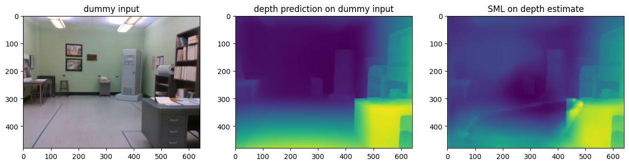
Storing and visualizing dummy results obtained
# Base directory in which outputs would be stored as a pathlib.Path variable
OUTPUT_DIR = Path('output')

# Create the output directory adjacent to the notebook and suppress errors if the directory already exists
OUTPUT_DIR.mkdir(exist_ok=True)

# Utility functions are directly available in modules.midas.utils
# Provide path names without any extension and let the write_depth
# function provide them for you. Take note of the arguments.
utils.write_depth(path=str(OUTPUT_DIR / 'dummy_input'), depth=d_depth, bits=2)
utils.write_depth(path=str(OUTPUT_DIR / 'dummy_input_sml'), depth=sml_pred_dummy, bits=2)
plt.figure()

img_dummy_in = mpimg.imread('data/image/dummy_img.png')
img_dummy_out = mpimg.imread(OUTPUT_DIR / 'dummy_input.png')
img_dummy_sml_out = mpimg.imread(OUTPUT_DIR / 'dummy_input_sml.png')

f, axes = plt.subplots(1, 3)
plt.subplots_adjust(right=2.0)

axes[0].imshow(img_dummy_in)
axes[1].imshow(img_dummy_out)
axes[2].imshow(img_dummy_sml_out)

axes[0].set_title('dummy input')
axes[1].set_title('depth prediction on dummy input')
axes[2].set_title('SML on depth estimate')
Text(0.5, 1.0, 'SML on depth estimate')
<Figure size 640x480 with 0 Axes>
Running inference on a test image
Now role of both the dummy inputs i.e. the dummy image as well as its associated depth map is now over. Since we have access to the compiled models now, we can load the one image available to us for pure inferencing purposes and run all the above steps one by one till plotting of the depth map.
If you haven’t noticed already the data directory of this tutorial has been arranged as follows. This allows us to comply to these rules.
data
├── image
│   ├── dummy_img.png       # RGB images
│   └── <timestamp>.png
└── sparse_depth
    ├── dummy_img.png       # sparse metric depth maps
    └── <timestamp>.png     # as 16b PNG files
At the same time, the depth storage method used in the VOID dataset is assumed.
If you are thinking of the file name format of the image for inference, here is the reasoning.
The dataset was collected using the Intel RealSense D435i camera, which was configured to produce synchronized accelerometer and gyroscope measurements at 400 Hz, along with synchronized VGA-size (640 x 480) RGB and depth streams at 30 Hz. The depth frames are acquired using active stereo and is aligned to the RGB frame using the sensor factory calibration. The frequency of sensor and depth stream input run at certain fixed frequencies and hence time stamping every frame captured is beneficial for maintaining structure as well as for debugging purposes later.
The image for inference and it sparse depth map is taken from the compressed dataset presenthere
# As before download the sample images for inference and take note of the image hashes if you
# want to use them later
download_file('https://user-images.githubusercontent.com/22426058/254174393-fc6dcc5f-f677-4618-b2ef-22e8e5cb1ebe.png', filename='1552097950.2672.png', directory=Path(DATA_DIR / 'image'), silent=True)
download_file('https://user-images.githubusercontent.com/22426058/254174379-5d00b66b-57b4-4e96-91e9-36ef15ec5a0a.png', filename='1552097950.2672.png', directory=Path(DATA_DIR / 'sparse_depth'), silent=True)

# Load the image and its depth scale
img_input = data_loader.load_input_image('data/image/1552097950.2672.png')
img_depth_input = data_loader.load_sparse_depth('data/sparse_depth/1552097950.2672.png')

# Transform the input image for the depth model
transformed_image = transform_image_for_depth(input_image=img_input, depth_model_transform=depth_model_transform)

# Run the depth model on the transformed input
depth_pred = run_depth_model(input_image_h=IMAGE_H, input_image_w=IMAGE_W,
                             transformed_image=transformed_image, compiled_depth_model=compiled_depth_model)


# Call the function on the sparse depth map
# with all default settings and store in appropriate variables
int_depth, int_scales = compute_global_scale_and_shift(input_sparse_depth=img_depth_input, validity_map=None, depth_pred=depth_pred)

# Transform the input image for the ScaleMapLearner model
transformed_image_scale = transform_image_for_depth_scale(input_image=img_input,
                                                          scale_map_learner_transform=scale_map_learner_transform,
                                                          int_depth=int_depth, int_scales=int_scales)

# Run the SML model using the set of inputs
sml_pred = run_depth_scale_model(input_image_h=IMAGE_H, input_image_w=IMAGE_W,
                                 transformed_image_for_depth_scale=transformed_image_scale,
                                 compiled_scale_map_learner=compiled_scale_map_learner)
data/image/1552097950.2672.png: 0%| | 0.00/371k [00:00<?, ?B/s]
data/sparse_depth/1552097950.2672.png: 0%| | 0.00/3.07k [00:00<?, ?B/s]
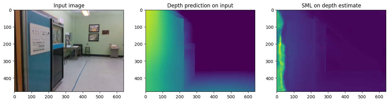
Store and visualize Inference results
# Store the depth and SML predictions
utils.write_depth(path=str(OUTPUT_DIR / '1552097950.2672'), depth=int_depth, bits=2)
utils.write_depth(path=str(OUTPUT_DIR / '1552097950.2672_sml'), depth=sml_pred, bits=2)


# Display result
plt.figure()

img_in = mpimg.imread('data/image/1552097950.2672.png')
img_out = mpimg.imread(OUTPUT_DIR / '1552097950.2672.png')
img_sml_out = mpimg.imread(OUTPUT_DIR / '1552097950.2672_sml.png')

f, axes = plt.subplots(1, 3)
plt.subplots_adjust(right=2.0)

axes[0].imshow(img_in)
axes[1].imshow(img_out)
axes[2].imshow(img_sml_out)

axes[0].set_title('Input image')
axes[1].set_title('Depth prediction on input')
axes[2].set_title('SML on depth estimate')
Text(0.5, 1.0, 'SML on depth estimate')
<Figure size 640x480 with 0 Axes>
Cleaning up the data directory
We will follow suit for the directory in which we downloaded images and depth maps from another repo. We shall move remove the unnecessary directories and files which were created during the download process.
# Remove the data directory and suppress errors(if any)
rmtree(path=str(DATA_DIR), ignore_errors=True)
Concluding notes
The code for this tutorial is adapted from the VI-Depth repository.
Users may choose to download the original and raw datasets from the VOID dataset.
The isl-org/VI-Depth works on a slightly older version of released model assets from its MiDaS sibling repository. However, the new releases beginning from v3.1 directly have OpenVINO™
.xmland.binmodel files as their assets thereby rendering the major pre-processing and model compilation step irrelevant.