Language-Visual Saliency with CLIP and OpenVINO™#
This Jupyter notebook can be launched on-line, opening an interactive environment in a browser window. You can also make a local installation. Choose one of the following options:
The notebook will cover the following topics:
Explanation of a saliency map and how it can be used.
Overview of the CLIP neural network and its usage in generating saliency maps.
How to split a neural network into parts for separate inference.
How to speed up inference with OpenVINO™ and asynchronous execution.
Saliency Map#
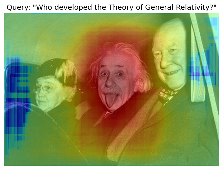
A saliency map is a visualization technique that highlights regions of interest in an image. For example, it can be used to explain image classification predictions for a particular label. Here is an example of a saliency map that you will get in this notebook:
CLIP#
What Is CLIP?#
CLIP (Contrastive Language–Image Pre-training) is a neural network that can work with both images and texts. It has been trained to predict which randomly sampled text snippets are close to a given image, meaning that a text better describes the image. Here is a visualization of the pre-training process:
To solve the task, CLIP uses two parts: Image Encoder and
Text Encoder. Both parts are used to produce embeddings, which are
vectors of floating-point numbers, for images and texts, respectively.
Given two vectors, one can define and measure the similarity between
them. A popular method to do so is the cosine_similarity, which is
defined as the dot product of the two vectors divided by the product of
their norms:

cs#
The result can range from \(-1\) to \(1\). A value \(1\) means that the vectors are similar, \(0\) means that the vectors are not “connected” at all, and \(-1\) is for vectors with somehow opposite “meaning”. To train CLIP, OpenAI uses samples of texts and images and organizes them so that the first text corresponds to the first image in the batch, the second text to the second image, and so on. Then, cosine similarities are measured between all texts and all images, and the results are put in a matrix. If the matrix has numbers close to \(1\) on a diagonal and close to \(0\) elsewhere, it indicates that the network is appropriately trained.
How to Build a Saliency Map with CLIP?#
Providing an image and a text to CLIP returns two vectors. The cosine similarity between these vectors is calculated, resulting in a number between \(-1\) and \(1\) that indicates whether the text describes the image or not. The idea is that some regions of the image are closer to the text query than others, and this difference can be used to build the saliency map. Here is how it can be done:
Compute
queryandimagesimilarity. This will represent the neutral value \(s_0\) on thesaliency map.Get a random
cropof the image.Compute
cropandquerysimilarity.Subtract the \(s_0\) from it. If the value is positive, the
cropis closer to thequery, and it should be a red region on the saliency map. If negative, it should be blue.Update the corresponding region on the
saliency map.Repeat steps 2-5 multiple times (
n_iters).
Table of contents:
Installation Instructions#
This is a self-contained example that relies solely on its own code.
We recommend running the notebook in a virtual environment. You only need a Jupyter server to start. For details, please refer to Installation Guide.
Initial Implementation with Transformers and Pytorch#
# Install requirements
%pip install -q "openvino>=2023.1.0"
%pip install -q --extra-index-url https://download.pytorch.org/whl/cpu transformers "numpy<2" "torch>=2.1" "gradio>=4.19" "matplotlib>=3.4"
from pathlib import Path
from typing import Tuple, Union, Optional
import requests

from matplotlib import colors
import matplotlib.pyplot as plt
import numpy as np
import torch
import tqdm
from PIL import Image
from transformers import CLIPModel, CLIPProcessor

if not Path("notebook_utils.py").exists():
    r = requests.get(
        url="https://raw.githubusercontent.com/openvinotoolkit/openvino_notebooks/latest/utils/notebook_utils.py",
    )
    open("notebook_utils.py", "w").write(r.text)

# Read more about telemetry collection at https://github.com/openvinotoolkit/openvino_notebooks?tab=readme-ov-file#-telemetry
from notebook_utils import collect_telemetry

collect_telemetry("clip-language-saliency-map.ipynb")
To get the CLIP model, you will use the transformers library and the
official openai/clip-vit-base-patch16 from OpenAI. You can use any
CLIP model from the HuggingFace Hub by simply replacing a model
checkpoint in the cell below.
There are several preprocessing steps required to get text and image
data to the model. Images have to be resized, cropped, and normalized,
and text must be split into tokens and swapped by token IDs. To do that,
you will use CLIPProcessor, which encapsulates all the preprocessing
steps.
model_checkpoint = "openai/clip-vit-base-patch16"

model = CLIPModel.from_pretrained(model_checkpoint).eval()
processor = CLIPProcessor.from_pretrained(model_checkpoint)
Let us write helper functions first. You will generate crop coordinates
and size with get_random_crop_params, and get the actual crop with
get_crop_image. To update the saliency map with the calculated
similarity, you will use update_saliency_map. A
cosine_similarity function is just a code representation of the
formula above.
def get_random_crop_params(image_height: int, image_width: int, min_crop_size: int) -> Tuple[int, int, int, int]:
    crop_size = np.random.randint(min_crop_size, min(image_height, image_width))
    x = np.random.randint(image_width - crop_size + 1)
    y = np.random.randint(image_height - crop_size + 1)
    return x, y, crop_size


def get_cropped_image(im_tensor: np.array, x: int, y: int, crop_size: int) -> np.array:
    return im_tensor[y : y + crop_size, x : x + crop_size, ...]


def update_saliency_map(saliency_map: np.array, similarity: float, x: int, y: int, crop_size: int) -> None:
    saliency_map[
        y : y + crop_size,
        x : x + crop_size,
    ] += similarity


def cosine_similarity(one: Union[np.ndarray, torch.Tensor], other: Union[np.ndarray, torch.Tensor]) -> Union[np.ndarray, torch.Tensor]:
    return one @ other.T / (np.linalg.norm(one) * np.linalg.norm(other))
Parameters to be defined:
n_iters- number of times the procedure will be repeated. Larger is better, but will require more time to inferencemin_crop_size- minimum size of the crop window. A smaller size will increase the resolution of the saliency map but may require more iterationsquery- text that will be used to query the imageimage- the actual image that will be queried. You will download the image from a link
The image at the beginning was acquired with n_iters=2000 and
min_crop_size=50. You will start with the lower number of inferences
to get the result faster. It is recommended to experiment with the
parameters at the end, when you get an optimized model.
n_iters = 300
min_crop_size = 50

query = "Who developed the Theory of General Relativity?"
image_path = Path("example.jpg")

if not image_path.exists():
    r = requests.get("https://github.com/user-attachments/assets/a5bedef2-e915-4286-bcc9-d599083a99a6")

    with image_path.open("wb") as f:
        f.write(r.content)
image = Image.open(image_path)
im_tensor = np.array(image)

x_dim, y_dim = image.size
Given the model and processor, the actual inference is simple:
transform the text and image into combined inputs and pass it to the
model:
inputs = processor(text=[query], images=[im_tensor], return_tensors="pt")
with torch.no_grad():
    results = model(**inputs)
results.keys()
odict_keys(['logits_per_image', 'logits_per_text', 'text_embeds', 'image_embeds', 'text_model_output', 'vision_model_output'])
The model produces several outputs, but for your application, you are
interested in text_embeds and image_embeds, which are the
vectors for text and image, respectively. Now, you can calculate
initial_similarity between the query and the image. You also
initialize a saliency map. Numbers in the comments correspond to the
items in the “How To Build a Saliency Map With CLIP?” list above.
initial_similarity = cosine_similarity(results.text_embeds, results.image_embeds).item()  # 1. Computing query and image similarity
saliency_map = np.zeros((y_dim, x_dim))

for _ in tqdm.notebook.tqdm(range(n_iters)):  # 6. Setting number of the procedure iterations
    x, y, crop_size = get_random_crop_params(y_dim, x_dim, min_crop_size)
    im_crop = get_cropped_image(im_tensor, x, y, crop_size)  # 2. Getting a random crop of the image

    inputs = processor(text=[query], images=[im_crop], return_tensors="pt")
    with torch.no_grad():
        results = model(**inputs)  # 3. Computing crop and query similarity

    similarity = (
        cosine_similarity(results.text_embeds, results.image_embeds).item() - initial_similarity
    )  # 4. Subtracting query and image similarity from crop and query similarity
    update_saliency_map(saliency_map, similarity, x, y, crop_size)  # 5. Updating the region on the saliency map
0%| | 0/300 [00:00<?, ?it/s]
To visualize the resulting saliency map, you can use matplotlib:
plt.figure(dpi=150)
plt.imshow(saliency_map, norm=colors.TwoSlopeNorm(vcenter=0), cmap="jet")
plt.colorbar(location="bottom")
plt.title(f'Query: "{query}"')
plt.axis("off")
plt.show()
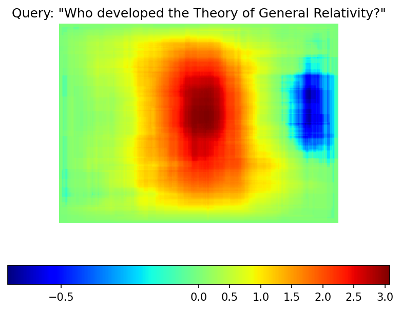
The result map is not as smooth as in the example picture because of the lower number of iterations. However, the same red and blue areas are clearly visible.
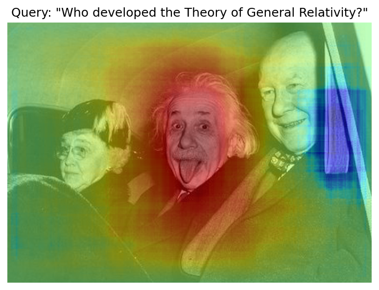
Let us overlay the saliency map on the image:
def plot_saliency_map(image_tensor: np.ndarray, saliency_map: np.ndarray, query: Optional[str]) -> None:
    fig = plt.figure(dpi=150)
    plt.imshow(image_tensor)
    plt.imshow(
        saliency_map,
        norm=colors.TwoSlopeNorm(vcenter=0),
        cmap="jet",
        alpha=0.5,  # make saliency map trasparent to see original picture
    )
    if query:
        plt.title(f'Query: "{query}"')
    plt.axis("off")
    return fig


plot_saliency_map(im_tensor, saliency_map, query);
Separate Text and Visual Processing#
The code above is functional, but there are some repeated computations
that can be avoided. The text embedding can be computed once because it
does not depend on the input image. This separation will also be useful
in the future. The initial preparation will remain the same since you
still need to compute the similarity between the text and the full
image. After that, the get_image_features method could be used to
obtain embeddings for the cropped images.
inputs = processor(text=[query], images=[im_tensor], return_tensors="pt")
with torch.no_grad():
    results = model(**inputs)
text_embeds = results.text_embeds  # save text embeddings to use them later

initial_similarity = cosine_similarity(text_embeds, results.image_embeds).item()
saliency_map = np.zeros((y_dim, x_dim))

for _ in tqdm.notebook.tqdm(range(n_iters)):
    x, y, crop_size = get_random_crop_params(y_dim, x_dim, min_crop_size)
    im_crop = get_cropped_image(im_tensor, x, y, crop_size)

    image_inputs = processor(images=[im_crop], return_tensors="pt")  # crop preprocessing
    with torch.no_grad():
        image_embeds = model.get_image_features(**image_inputs)  # calculate image embeddings only

    similarity = cosine_similarity(text_embeds, image_embeds).item() - initial_similarity
    update_saliency_map(saliency_map, similarity, x, y, crop_size)

plot_saliency_map(im_tensor, saliency_map, query);
0%| | 0/300 [00:00<?, ?it/s]
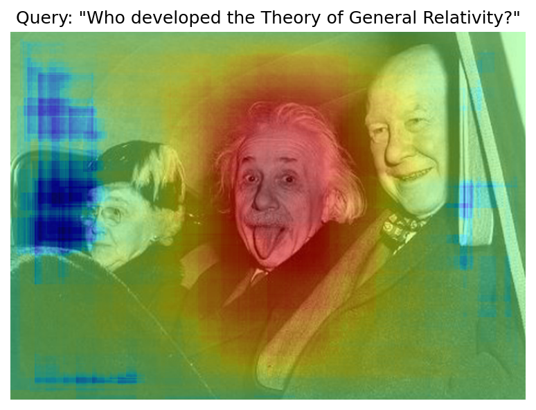
The result might be slightly different because you use random crops to build a saliency map.
Convert to OpenVINO™ Intermediate Representation (IR) Format#
The process of building a saliency map can be quite time-consuming. To
speed it up, you will use OpenVINO. OpenVINO is an inference framework
designed to run pre-trained neural networks efficiently. One way to use
it is to convert a model from its original framework representation to
an OpenVINO Intermediate Representation (IR) format and then load it for
inference. The model currently uses PyTorch. To get an IR, you need to
use Model Conversion API. ov.convert_model function accepts PyTorch
model object and example input and converts it to OpenVINO Model
instance, that ready to load on device using ov.compile_model or can
be saved on disk using ov.save_model. To separate model on text and
image parts, we overload forward method with get_text_features and
get_image_features methods respectively. Internally, PyTorch
conversion to OpenVINO involves TorchScript tracing. For achieving
better conversion results, we need to guarantee that model can be
successfully traced. model.config.torchscript = True parameters
allows to prepare HuggingFace models for TorchScript tracing. More
details about that can be found in HuggingFace Transformers
documentation
import openvino as ov

model_name = model_checkpoint.split("/")[-1]

model.config.torchscript = True
model.forward = model.get_text_features
text_ov_model = ov.convert_model(
    model,
    example_input={
        "input_ids": inputs.input_ids,
        "attention_mask": inputs.attention_mask,
    },
)

# get image size after preprocessing from the processor
crops_info = processor.image_processor.crop_size.values() if hasattr(processor, "image_processor") else processor.feature_extractor.crop_size.values()
model.forward = model.get_image_features
image_ov_model = ov.convert_model(
    model,
    example_input={"pixel_values": inputs.pixel_values},
    input=[1, 3, *crops_info],
)

ov_dir = Path("ir")
ov_dir.mkdir(exist_ok=True)
text_model_path = ov_dir / f"{model_name}_text.xml"
image_model_path = ov_dir / f"{model_name}_image.xml"

# write resulting models on disk
ov.save_model(text_ov_model, text_model_path)
ov.save_model(image_ov_model, image_model_path)
WARNING:tensorflow:Please fix your imports. Module tensorflow.python.training.tracking.base has been moved to tensorflow.python.trackable.base. The old module will be deleted in version 2.11.
[ WARNING ] Please fix your imports. Module %s has been moved to %s. The old module will be deleted in version %s.
INFO:nncf:NNCF initialized successfully. Supported frameworks detected: torch, tensorflow, onnx, openvino
huggingface/tokenizers: The current process just got forked, after parallelism has already been used. Disabling parallelism to avoid deadlocks...
To disable this warning, you can either:
    - Avoid using tokenizers before the fork if possible
    - Explicitly set the environment variable TOKENIZERS_PARALLELISM=(true | false)
huggingface/tokenizers: The current process just got forked, after parallelism has already been used. Disabling parallelism to avoid deadlocks...
To disable this warning, you can either:
    - Avoid using tokenizers before the fork if possible
    - Explicitly set the environment variable TOKENIZERS_PARALLELISM=(true | false)
huggingface/tokenizers: The current process just got forked, after parallelism has already been used. Disabling parallelism to avoid deadlocks...
To disable this warning, you can either:
    - Avoid using tokenizers before the fork if possible
    - Explicitly set the environment variable TOKENIZERS_PARALLELISM=(true | false)
No CUDA runtime is found, using CUDA_HOME='/usr/local/cuda'
/home/ea/work/ov_venv/lib/python3.8/site-packages/transformers/models/clip/modeling_clip.py:287: TracerWarning: Converting a tensor to a Python boolean might cause the trace to be incorrect. We can't record the data flow of Python values, so this value will be treated as a constant in the future. This means that the trace might not generalize to other inputs!
  if attn_weights.size() != (bsz * self.num_heads, tgt_len, src_len):
/home/ea/work/ov_venv/lib/python3.8/site-packages/transformers/models/clip/modeling_clip.py:295: TracerWarning: Converting a tensor to a Python boolean might cause the trace to be incorrect. We can't record the data flow of Python values, so this value will be treated as a constant in the future. This means that the trace might not generalize to other inputs!
  if causal_attention_mask.size() != (bsz, 1, tgt_len, src_len):
/home/ea/work/ov_venv/lib/python3.8/site-packages/transformers/models/clip/modeling_clip.py:304: TracerWarning: Converting a tensor to a Python boolean might cause the trace to be incorrect. We can't record the data flow of Python values, so this value will be treated as a constant in the future. This means that the trace might not generalize to other inputs!
  if attention_mask.size() != (bsz, 1, tgt_len, src_len):
/home/ea/work/ov_venv/lib/python3.8/site-packages/transformers/models/clip/modeling_clip.py:327: TracerWarning: Converting a tensor to a Python boolean might cause the trace to be incorrect. We can't record the data flow of Python values, so this value will be treated as a constant in the future. This means that the trace might not generalize to other inputs!
  if attn_output.size() != (bsz * self.num_heads, tgt_len, self.head_dim):
Now, you have two separate models for text and images, stored on disk and ready to be loaded and inferred with OpenVINO™.
Inference with OpenVINO™#
Create an instance of the
Coreobject that will handle any interaction with OpenVINO runtime for you.Use the
core.read_modelmethod to load the model into memory.Compile the model with the
core.compile_modelmethod for a particular device to apply device-specific optimizations.Use the compiled model for inference.
core = ov.Core()

text_model = core.read_model(text_model_path)
image_model = core.read_model(image_model_path)
Select inference device#
select device from dropdown list for running inference using OpenVINO
from notebook_utils import device_widget

device = device_widget()

device
Dropdown(description='Device:', index=2, options=('CPU', 'GPU', 'AUTO'), value='AUTO')
text_model = core.compile_model(model=text_model, device_name=device.value)
image_model = core.compile_model(model=image_model, device_name=device.value)
OpenVINO supports numpy.ndarray as an input type, so you change the
return_tensors to np. You also convert a transformers’
BatchEncoding object to a python dictionary with input names as keys
and input tensors for values.
Once you have a compiled model, the inference is similar to Pytorch - a compiled model is callable. Just pass input data to it. Inference results are stored in the dictionary. Once you have a compiled model, the inference process is mostly similar.
text_inputs = dict(processor(text=[query], images=[im_tensor], return_tensors="np"))
image_inputs = text_inputs.pop("pixel_values")

text_embeds = text_model(text_inputs)[0]
image_embeds = image_model(image_inputs)[0]

initial_similarity = cosine_similarity(text_embeds, image_embeds)
saliency_map = np.zeros((y_dim, x_dim))

for _ in tqdm.notebook.tqdm(range(n_iters)):
    x, y, crop_size = get_random_crop_params(y_dim, x_dim, min_crop_size)
    im_crop = get_cropped_image(im_tensor, x, y, crop_size)

    image_inputs = processor(images=[im_crop], return_tensors="np").pixel_values
    image_embeds = image_model(image_inputs)[image_model.output()]

    similarity = cosine_similarity(text_embeds, image_embeds) - initial_similarity
    update_saliency_map(saliency_map, similarity, x, y, crop_size)

plot_saliency_map(im_tensor, saliency_map, query);
0%| | 0/300 [00:00<?, ?it/s]
Accelerate Inference with AsyncInferQueue#
Up until now, the pipeline was synchronous, which means that the data
preparation, model input population, model inference, and output
processing is sequential. That is a simple, but not the most effective
way to organize an inference pipeline in your case. To utilize the
available resources more efficiently, you will use AsyncInferQueue.
It can be instantiated with compiled model and a number of jobs -
parallel execution threads. If you do not pass a number of jobs or pass
0, then OpenVINO will pick the optimal number based on your device
and heuristics. After acquiring the inference queue, you have two jobs
to do:
Preprocess the data and push it to the inference queue. The preprocessing steps will remain the same
Tell the inference queue what to do with the model output after the inference is finished. It is represented by a python function called
callbackthat takes an inference result and data that you passed to the inference queue along with the prepared input data
Everything else will be handled by the AsyncInferQueue instance.
There is another low-hanging bit of optimization. You are expecting many inference requests for your image model at once and want the model to process them as fast as possible. In other words - maximize the throughput. To do that, you can recompile the model giving it the performance hint.
from typing import Dict, Any
import openvino.properties.hint as hints


image_model = core.read_model(image_model_path)

image_model = core.compile_model(
    model=image_model,
    device_name=device.value,
    config={hints.performance_mode(): hints.PerformanceMode.THROUGHPUT},
)
text_inputs = dict(processor(text=[query], images=[im_tensor], return_tensors="np"))
image_inputs = text_inputs.pop("pixel_values")

text_embeds = text_model(text_inputs)[text_model.output()]
image_embeds = image_model(image_inputs)[image_model.output()]

initial_similarity = cosine_similarity(text_embeds, image_embeds)
saliency_map = np.zeros((y_dim, x_dim))
Your callback should do the same thing that you did after inference in the sync mode:
Pull the image embeddings from an inference request.
Compute cosine similarity between text and image embeddings.
Update saliency map based.
If you do not change the progress bar, it will show the progress of
pushing data to the inference queue. To track the actual progress, you
should pass a progress bar object and call update method after
update_saliency_map call.
def completion_callback(
    infer_request: ov.InferRequest,  # inferente result
    user_data: Dict[str, Any],  # data that you passed along with input pixel values
) -> None:
    pbar = user_data.pop("pbar")

    image_embeds = infer_request.get_output_tensor().data
    similarity = cosine_similarity(user_data.pop("text_embeds"), image_embeds) - user_data.pop("initial_similarity")
    update_saliency_map(**user_data, similarity=similarity)

    pbar.update(1)  # update the progress bar


infer_queue = ov.AsyncInferQueue(image_model)
infer_queue.set_callback(completion_callback)
def infer(
    im_tensor,
    x_dim,
    y_dim,
    text_embeds,
    image_embeds,
    initial_similarity,
    saliency_map,
    query,
    n_iters,
    min_crop_size,
    _tqdm=tqdm.notebook.tqdm,
    include_query=True,
):
    with _tqdm(total=n_iters) as pbar:
        for _ in range(n_iters):
            x, y, crop_size = get_random_crop_params(y_dim, x_dim, min_crop_size)
            im_crop = get_cropped_image(im_tensor, x, y, crop_size)

            image_inputs = processor(images=[im_crop], return_tensors="np")

            # push data to the queue
            infer_queue.start_async(
                # pass inference data as usual
                image_inputs.pixel_values,
                # the data that will be passed to the callback after the inference complete
                {
                    "text_embeds": text_embeds,
                    "saliency_map": saliency_map,
                    "initial_similarity": initial_similarity,
                    "x": x,
                    "y": y,
                    "crop_size": crop_size,
                    "pbar": pbar,
                },
            )

        # after you pushed all data to the queue you wait until all callbacks finished
        infer_queue.wait_all()

    return plot_saliency_map(im_tensor, saliency_map, query if include_query else None)


infer(
    im_tensor,
    x_dim,
    y_dim,
    text_embeds,
    image_embeds,
    initial_similarity,
    saliency_map,
    query,
    n_iters,
    min_crop_size,
    _tqdm=tqdm.notebook.tqdm,
    include_query=True,
);
0%| | 0/300 [00:00<?, ?it/s]
Pack the Pipeline into a Function#
Let us wrap all code in the function and add a user interface to it.
import ipywidgets as widgets


def build_saliency_map(
    image: Image,
    query: str,
    n_iters: int = n_iters,
    min_crop_size=min_crop_size,
    _tqdm=tqdm.notebook.tqdm,
    include_query=True,
):
    x_dim, y_dim = image.size
    im_tensor = np.array(image)

    text_inputs = dict(processor(text=[query], images=[im_tensor], return_tensors="np"))
    image_inputs = text_inputs.pop("pixel_values")

    text_embeds = text_model(text_inputs)[text_model.output()]
    image_embeds = image_model(image_inputs)[image_model.output()]

    initial_similarity = cosine_similarity(text_embeds, image_embeds)
    saliency_map = np.zeros((y_dim, x_dim))

    return infer(
        im_tensor,
        x_dim,
        y_dim,
        text_embeds,
        image_embeds,
        initial_similarity,
        saliency_map,
        query,
        n_iters,
        min_crop_size,
        _tqdm=_tqdm,
        include_query=include_query,
    )
The first version will enable passing a link to the image, as you have done so far in the notebook.
n_iters_widget = widgets.BoundedIntText(
    value=n_iters,
    min=1,
    max=10000,
    description="n_iters",
)
min_crop_size_widget = widgets.IntSlider(
    value=min_crop_size,
    min=1,
    max=200,
    description="min_crop_size",
)


@widgets.interact_manual(image_link="", query="", n_iters=n_iters_widget, min_crop_size=min_crop_size_widget)
def build_saliency_map_from_image_link(
    image_link: str,
    query: str,
    n_iters: int,
    min_crop_size: int,
) -> None:
    try:
        image_bytes = requests.get(image_link, stream=True).raw
    except requests.RequestException as e:
        print(f"Cannot load image from link: {image_link}\nException: {e}")
        return

    image = Image.open(image_bytes)
    image = image.convert("RGB")  # remove transparency channel or convert grayscale 1 channel to 3 channels

    build_saliency_map(image, query, n_iters, min_crop_size)
interactive(children=(Text(value='', continuous_update=False, description='image_link'), Text(value='', contin…
The second version will enable loading the image from your computer.
import io


load_file_widget = widgets.FileUpload(
    accept="image/*",
    multiple=False,
    description="Image file",
)


@widgets.interact_manual(
    file=load_file_widget,
    query="",
    n_iters=n_iters_widget,
    min_crop_size=min_crop_size_widget,
)
def build_saliency_map_from_file(
    file: Path,
    query: str = "",
    n_iters: int = 2000,
    min_crop_size: int = 50,
) -> None:
    image_bytes = io.BytesIO(file[0]["content"])
    try:
        image = Image.open(image_bytes)
    except Exception as e:
        print(f"Cannot load the image: {e}")
        return

    image = image.convert("RGB")

    build_saliency_map(image, query, n_iters, min_crop_size)
interactive(children=(FileUpload(value=(), accept='image/*', description='Image file'), Text(value='', continu…
Interactive demo with Gradio#
if not Path("gradio_helper.py").exists():
    r = requests.get(url="https://raw.githubusercontent.com/openvinotoolkit/openvino_notebooks/latest/notebooks/clip-language-saliency-map/gradio_helper.py")
    open("gradio_helper.py", "w").write(r.text)

from gradio_helper import make_demo

demo = make_demo(build_saliency_map)

try:
    demo.queue().launch(debug=False)
except Exception:
    demo.queue().launch(share=True, debug=False)
# if you are launching remotely, specify server_name and server_port
# demo.launch(server_name='your server name', server_port='server port in int')
# Read more in the docs: https://gradio.app/docs/
Running on local URL:  http://127.0.0.1:7860

To create a public link, set share=True in launch().
What To Do Next#
Now that you have a convenient interface and accelerated inference, you can explore the CLIP capabilities further. For example:
Can CLIP read? Can it detect text regions in general and specific words on the image?
Which famous people and places does CLIP know?
Can CLIP identify places on a map? Or planets, stars, and constellations?
Explore different CLIP models from HuggingFace Hub: just change the
model_checkpointat the beginning of the notebook.Add batch processing to the pipeline: modify
get_random_crop_params,get_cropped_imageandupdate_saliency_mapfunctions to process multiple crop images at once and accelerate the pipeline even more.Optimize models with NNCF to get further acceleration. You can find example how to quantize CLIP model in this notebook