OpenVINO™ Explainable AI Toolkit (3/3): Saliency map interpretation#
This Jupyter notebook can be launched on-line, opening an interactive environment in a browser window. You can also make a local installation. Choose one of the following options:


Warning
Important note: This notebook requires python >= 3.10. Please make sure that your environment fulfill to this requirement before running it
This is the third notebook in series of exploring OpenVINO™ Explainable AI (XAI):
OpenVINO™ Explainable AI (XAI) provides a suite of XAI algorithms for visual explanation of OpenVINO™ Intermediate Representation (IR) models.
Using OpenVINO XAI, you can generate saliency maps that highlight regions of interest in input images from the model’s perspective. This helps users understand why complex AI models produce specific responses.
This notebook shows how to use saliency maps to evaluate and debug model reasoning.
For example, it might be important to ensure that the model is using relevant features (pixels) to make a correct prediction (e.g., it might be desirable that the model is not relying on X class features to predict Y class). On the other hand, it is valuable to observe which features are used when the model is wrong.
Below, we present examples of saliency map analysis for the following cases: correct and highly-confident prediction, correct and low-confident prediction, and wrong prediction.
Table of contents:
Installation Instructions#
This is a self-contained example that relies solely on its own code.
We recommend running the notebook in a virtual environment. You only need a Jupyter server to start. For details, please refer to Installation Guide.
Prerequisites#
Install requirements#
%%capture

import platform

# Install openvino package
%pip install -q "openvino>=2024.2.0" opencv-python tqdm

# Install openvino xai package
%pip install -q --no-deps "openvino-xai>=1.1.0"
%pip install -q -U "numpy==1.*"
%pip install -q scipy

%pip install -q "matplotlib>=3.4"
Imports#
import os
import zipfile
from pathlib import Path

import cv2
import matplotlib.pyplot as plt
import numpy as np
import requests

import openvino.runtime as ov
import openvino_xai as xai
from openvino_xai.explainer import ExplainMode

if not Path("notebook_utils.py").exists():
    # Fetch `notebook_utils` module
    r = requests.get(
        url="https://raw.githubusercontent.com/openvinotoolkit/openvino_notebooks/latest/utils/notebook_utils.py",
    )

    open("notebook_utils.py", "w").write(r.text)

from notebook_utils import download_file, device_widget

# Read more about telemetry collection at https://github.com/openvinotoolkit/openvino_notebooks?tab=readme-ov-file#-telemetry
from notebook_utils import collect_telemetry

collect_telemetry("explainable-ai-3-map-interpretation.ipynb")
Download dataset#
To see examples of saliency maps for different use cases, please download the ImageWoof dataset using the code below.
ImageWoof is a subset of 10 classes from ImageNet that are tricky to classify since they’re all dog breeds.
base_artifacts_dir = Path("./artifacts").expanduser()
data_folder = base_artifacts_dir / ".data"
# Download 330 MB of 320 px ImageNet subset with dog breeds
if not (data_folder / "imagewoof320").exists():
    download_file(
        "https://ultralytics.com/assets/imagewoof320.zip",
        directory=data_folder,
    )

    # Define the path to the zip file and the destination directory
    zip_path = data_folder / "imagewoof320.zip"
    extract_dir = data_folder / "imagewoof320"
    with zipfile.ZipFile(zip_path, "r") as zip_ref:
        zip_ref.extractall(extract_dir)

else:
    print(f"Dataset is already downloaded to {base_artifacts_dir} and extracted.")

image_folder_path = data_folder / "imagewoof320" / "imagewoof320"
# Create list of images to explain
img_files = []
img_files.extend(image_folder_path.rglob("*.JPEG"))
print(f"Number of images to get explanations: {len(img_files)}")

# Get a fewer subset for fast execution
np.random.seed(42)
img_files = np.random.choice(img_files, 1)
print(f"Run explanations on fewer number of images: {len(img_files)}")
Number of images to get explanations: 12954
Run explanations on fewer number of images: 1
Download IR model#
In this notebook, for demonstration purposes, we’ll use an already
converted to IR model mobilenetv3_large_100.ra_in1k, from
timm (PyTorch
Image Models). This model requires specific preprocessing, including
scaling and normalization with certain values.
model_name = "mobilenetv3_large_100.ra_in1k"
model_xml_name = f"{model_name}.xml"
model_bin_name = f"{model_name}.bin"

model_xml_path = base_artifacts_dir / model_xml_name

base_url = "https://storage.openvinotoolkit.org/repositories/openvino_training_extensions/models/custom_image_classification/"

if not model_xml_path.exists():
    download_file(base_url + model_xml_name, model_xml_name, base_artifacts_dir)
    download_file(base_url + model_bin_name, model_bin_name, base_artifacts_dir)
else:
    print(f"{model_name} already downloaded to {base_artifacts_dir}")
Prepare model to run inference#
Select inference device#
select device from dropdown list for running inference using OpenVINO
device = device_widget()

device
Load the Model#
core = ov.Core()

model = core.read_model(model=model_xml_path)
compiled_model = core.compile_model(model=model, device_name=device.value)
Define preprocess_fn#
This notebook using WHITEBOX mode for model explanation - it is
required to define function to preprocess data (the alternative is to
preprocess input data). Since the used model is originally from timm
storage, it is
required to apply specific timm preprocessing, including normalization
and scaling with certain values.
def preprocess_fn(x: np.ndarray) -> np.ndarray:
    """
    Implementing own pre-process function based on model's implementation
    """
    x = cv2.resize(src=x, dsize=(224, 224))

    #  Specific normalization for timm model
    mean = np.array([123.675, 116.28, 103.53])
    std = np.array([58.395, 57.12, 57.375])
    x = (x - std) / mean

    # Reshape to model input shape to [channels, height, width].
    x = x.transpose((2, 0, 1))

    # Add batch dimension
    x = np.expand_dims(x, 0)
    return x
Explain#
Create Explainer object#
The Explainer object can internally apply pre-processing during
model inference, allowing raw images as input. To enable this, define
preprocess_fn and provide it to the explainer constructor. If
preprocess_fn is not defined, it is assumed that the input is
preprocessed.
# Create ov.Model
model = core.read_model(model=model_xml_path)

# Create explainer object
explainer = xai.Explainer(
    model=model,
    task=xai.Task.CLASSIFICATION,
    preprocess_fn=preprocess_fn,
    explain_mode=ExplainMode.WHITEBOX,
)
INFO:openvino_xai:Target insertion layer is not provided - trying to find it in auto mode.
INFO:openvino_xai:Using ReciproCAM method (for CNNs).
INFO:openvino_xai:Explaining the model in white-box mode.
Import ImageNet label names#
If label_names are not provided to the explainer call, the saved
saliency map will have the predicted class index, not the name. For
example, 167.jpg instead of English_foxhound.jpg.
To conveniently view label names in saliency maps, we prepare and provide ImageNet label names information to the explanation call.
%%capture
imagenet_filename = Path(".data/imagenet_2012.txt")
if not imagenet_filename.exists():
    imagenet_filename = download_file(
        "https://storage.openvinotoolkit.org/repositories/openvino_notebooks/data/data/datasets/imagenet/imagenet_2012.txt",
        directory=".data",
    )

imagenet_classes = imagenet_filename.read_text().splitlines()
# Get ImageNet label names to add them to explanations
imagenet_labels = []
for label in imagenet_classes:
    class_label = " ".join(label.split(" ")[1:])
    first_class_label = class_label.split(",")[0].replace(" ", "_")
    imagenet_labels.append(first_class_label)

# Check, how dog breed labels will look in saved saliency map names
dog_breeds_indices = [155, 159, 162, 167, 193, 207, 229, 258, 273]
print(" ".join([imagenet_labels[ind] for ind in dog_breeds_indices]))
Shih-Tzu Rhodesian_ridgeback beagle English_foxhound Australian_terrier golden_retriever Old_English_sheepdog Samoyed dingo
Explain using ImageNet labels#
To use ImageNet label names, pass them as the label_names argument
to the explainer.
output = base_artifacts_dir / "saliency_maps" / "multiple_images"

# Explain model and save results using ImageNet label names
for image_path in img_files:
    image = cv2.imread(str(image_path))
    explanation = explainer(
        image,
        targets=[
            "flat-coated_retriever",
            "Samoyed",
        ],  # also label indices [206, 258] are possible as target
        label_names=imagenet_labels,
    )
    explanation.save(output, f"{Path(image_path).stem}_")  # pass prefix name with underscore
Below in base_artifacts_dir / "saliency_maps" / "multiple_images"
you can see saved saliency maps:
# See saliency that was saved in `output` with predicted label in image name
for file_name in output.glob("*"):
    print(file_name)
artifacts/saliency_maps/multiple_images/n02088364_5768_Samoyed.jpg
artifacts/saliency_maps/multiple_images/n02088364_5768_flat-coated_retriever.jpg
Notable use cases in ImageWoof dataset#
Below are a few examples chosen to show cases when: - The correct class
was predicted with high confidence (True Positive, high confidence)
- The correct class was predicted, but with low confidence for some
reason (True Positive, low confidence) - The predicted class has
high confidence but was incorrect, one class was treated as another
(False positive, high confidence) - Two classes were predicted with
similar high confidence, with different saliency maps for each
(Two predictions)
The cell below contains paths to images with those respective use cases:
# Read paths to ImegeWoof pictures with notable use cases
use_cases_image_paths = {
    "True_positive_high_confidence": {
        "confidence": 0.79,
        "paths": [
            "train/n02088364/n02088364_2019.JPEG",
            "train/n02099601/n02099601_6505.JPEG",
            "train/n02105641/n02105641_817.JPEG",
            "train/n02111889/n02111889_17737.JPEG",
        ],
    },
    "True_positive_low_confidence": {
        "confidence": 0.15,
        "paths": [
            "train/n02086240/n02086240_1765.JPEG",
            "val/n02086240/n02086240_1422.JPEG",
            "train/n02086240/n02086240_3709.JPEG",
            "val/n02099601/n02099601_7942.JPEG",
        ],
    },
    "False_positive_high_confidence": {
        "confidence": 0.60,
        "paths": [
            "train/n02087394/n02087394_6357.JPEG",
            "val/n02088364/n02088364_2430.JPEG",
            "train/n02088364/n02088364_12304.JPEG",
            "train/n02096294/n02096294_2323.JPEG",
            "train/n02099601/n02099601_4933.JPEG",
            "val/n02111889/n02111889_1931.JPEG",
            "train/n02111889/n02111889_14926.JPEG",
            "val/n02115641/n02115641_5752.JPEG",
        ],
    },
    "True_positive_two_predictions": {"confidence": 0.17, "paths": ["train/n02099601/n02099601_634.JPEG", "train/n02111889/n02111889_374.JPEG"]},
}
# Add mapping from folder name to label and label_idx to define the ground-truth label
label_mapping = {
    "n02088364": ("beagle", 162),
    "n02099601": ("golden retriever", 207),
    "n02105641": ("Old English sheepdog", 229),
    "n02111889": ("Samoyed", 258),
    "n02086240": ("Shih-Tzu", 155),
    "n02089973": ("English foxhound", 167),
    "n02087394": ("Rhodesian ridgeback", 159),
    "n02096294": ("Australian terrier", 193),
    "n02115641": ("dingo", 273),
}
def get_model_predictions(conf_thr: float = 0.1) -> tuple[np.ndarray, np.ndarray, np.ndarray]:
    """
    Run model inference and get predictions above a confidence threshold.

    Args:
        conf_thr (float): Confidence threshold for filtering predictions. Defaults to 0.1.

    Returns:
        tuple: A tuple containing:
            - result_infer (np.ndarray): The raw inference results from the model.
            - result_idxs (np.ndarray): Indices of the predictions above the confidence threshold.
            - result_scores (np.ndarray): Scores of the predictions above the confidence threshold.
    """
    logits = compiled_model([preprocess_fn(image)])[0]
    result_infer = postprocess_fn(logits)
    result_idxs = np.argwhere(result_infer > conf_thr).flatten()
    result_scores = result_infer[result_idxs]

    for index, score in zip(result_idxs, result_scores):
        print(f"Predicted class {imagenet_labels[index]}, index {index}, probability: {score:.2f}")

    return result_infer, result_idxs, result_scores


def postprocess_fn(x: np.ndarray) -> np.ndarray:
    """
    Process model prediction
    """
    prediction_processed = softmax(x)
    return prediction_processed[0]  # remove batch dimension


def softmax(x):
    """Compute softmax values of x."""
    e_x = np.exp(x - np.max(x))
    return e_x / e_x.sum()
Explain for each use case#
output = base_artifacts_dir / "saliency_maps" / "imagewoof320"

# Run explanation for chosen paths
for use_case in use_cases_image_paths:
    os.makedirs(output / use_case, exist_ok=True)
    image_paths = use_cases_image_paths[use_case]["paths"]
    use_case_conf_thr = use_cases_image_paths[use_case]["confidence"]

    for image_path in image_paths:
        image = cv2.imread(str(image_folder_path / image_path))
        image_name = Path(image_path).stem

        folder_name = image_name.split("_")[0]
        gt_class, gt_class_idx = label_mapping[folder_name]

        scores, result_idxs, result_scores = get_model_predictions(use_case_conf_thr)
        gt_conf = scores[gt_class_idx]
        gt_info = f"gt_{gt_class}_{gt_conf:.2f}"

        explanation = explainer(
            image,
            targets=result_idxs,  # return saliency maps for predicted classes
            label_names=imagenet_labels,
            overlay=True,
        )

        saliency_map_name_prefix = f"{image_name}_{gt_info}_pr_"
        saliency_map_name_postfix = "_"
        confidence_scores = {}
        for idx, score in zip(result_idxs, result_scores):
            confidence_scores[idx] = score
        explanation.save(
            dir_path=(output / use_case),
            prefix=saliency_map_name_prefix,
            postfix=saliency_map_name_postfix,
            confidence_scores=confidence_scores,
        )
Predicted class beagle, index 162, probability: 0.97
Predicted class golden_retriever, index 207, probability: 0.88
Predicted class Old_English_sheepdog, index 229, probability: 0.96
Predicted class Samoyed, index 258, probability: 0.94
Predicted class Shih-Tzu, index 155, probability: 0.18
Predicted class Shih-Tzu, index 155, probability: 0.18
Predicted class Shih-Tzu, index 155, probability: 0.20
Predicted class golden_retriever, index 207, probability: 0.18
Predicted class dalmatian, index 251, probability: 0.98
Predicted class bannister, index 421, probability: 0.78
Predicted class car_mirror, index 475, probability: 0.82
Predicted class quilt, index 750, probability: 0.80
Predicted class bubble, index 971, probability: 0.79
Predicted class dogsled, index 537, probability: 0.79
Predicted class Arctic_fox, index 279, probability: 0.95
Predicted class Chihuahua, index 151, probability: 0.93
Predicted class golden_retriever, index 207, probability: 0.30
Predicted class Labrador_retriever, index 208, probability: 0.57
Predicted class Samoyed, index 258, probability: 0.43
Predicted class crib, index 520, probability: 0.39
# Check saved saliency maps for debugging purposes
for use_case in use_cases_image_paths:
    print("\n", use_case)
    for file_name in (output / use_case).glob("*"):
        print(file_name.stem)
 True_positive_high_confidence
n02088364_2019_gt_beagle_0.97_pr_beagle_0.97
n02099601_6505_gt_golden retriever_0.88_pr_golden_retriever_0.88
n02105641_817_gt_Old English sheepdog_0.96_pr_Old_English_sheepdog_0.96
n02111889_17737_gt_Samoyed_0.94_pr_Samoyed_0.94

 True_positive_low_confidence
n02099601_7942_gt_golden retriever_0.18_pr_golden_retriever_0.18
n02086240_3709_gt_Shih-Tzu_0.20_pr_Shih-Tzu_0.20
n02086240_1422_gt_Shih-Tzu_0.18_pr_Shih-Tzu_0.18
n02086240_1765_gt_Shih-Tzu_0.18_pr_Shih-Tzu_0.18

 False_positive_high_confidence
n02088364_12304_gt_beagle_0.01_pr_car_mirror_0.82
n02088364_2430_gt_beagle_0.00_pr_bannister_0.78
n02099601_4933_gt_golden retriever_0.05_pr_bubble_0.79
n02096294_2323_gt_Australian terrier_0.00_pr_quilt_0.80
n02115641_5752_gt_dingo_0.02_pr_Chihuahua_0.93
n02111889_1931_gt_Samoyed_0.07_pr_dogsled_0.79
n02087394_6357_gt_Rhodesian ridgeback_0.00_pr_dalmatian_0.98
n02111889_14926_gt_Samoyed_0.03_pr_Arctic_fox_0.95

 True_positive_two_predictions
n02099601_634_gt_golden retriever_0.30_pr_golden_retriever_0.30
n02111889_374_gt_Samoyed_0.43_pr_Samoyed_0.43
n02099601_634_gt_golden retriever_0.30_pr_Labrador_retriever_0.57
n02111889_374_gt_Samoyed_0.43_pr_crib_0.39
See the list of use case names:
print(f"Names of use cases: {list(use_cases_image_paths.keys())}")
Names of use cases: ['True_positive_high_confidence', 'True_positive_low_confidence', 'False_positive_high_confidence', 'True_positive_two_predictions']
Visualize use case saliency maps#
The function below helps to visualize the results by creating a matrix of pictures, their names, and the confidence of predictions:
# Function to show result saliency maps for each use case
def show_use_case_image(use_case):
    use_case_output_dir = output / use_case

    image_paths = sorted(os.listdir(use_case_output_dir))
    number_images = len(image_paths)

    fig, axs = plt.subplots((number_images + 1) // 2, 2, figsize=(10, 10))
    fig.tight_layout()
    fig.suptitle(use_case)
    fig.subplots_adjust(top=0.92)
    axs = axs.flatten()

    for image_path, ax in zip(image_paths, axs):
        image_sal_map = cv2.imread(f"{use_case_output_dir}/{image_path}")
        image_sal_map = cv2.cvtColor(image_sal_map, cv2.COLOR_BGR2RGB)

        image_name = Path(image_path).stem
        image_name = image_name.replace("_target", "")
        image_name = "_".join(image_name.split("_")[1:])

        ax.imshow(image_sal_map)
        ax.set_title(f"{image_name}", wrap=True)
        ax.axis("off")

    if number_images % 2 == 1:
        axs[-1].set_visible(False)

    plt.show()
Naming logic#
The name of saved saliency maps in this notebook contains info about the
ground-truth class, predicted class, and its confidence. For better
understanding, let’s split the name into meaningful parts and learn its
meaning, taking 5752_gt_dingo_0.18_pr_Chihuahua_0.93 as an example.
5752 - the number of the image, truncated from the original name
n02115641_5752.
gt_dingo_0.18 - ground-truth info, the image was annotated as
the dingo class, and the model predicted this class with 0.18
confidence.
pr_Chihuahua_0.93 - predicted info, the winning class is
Chihuahua, and the model made this prediction with 0.93
confidence.
Results#
True Positive High confidence#
show_use_case_image("True_positive_high_confidence")
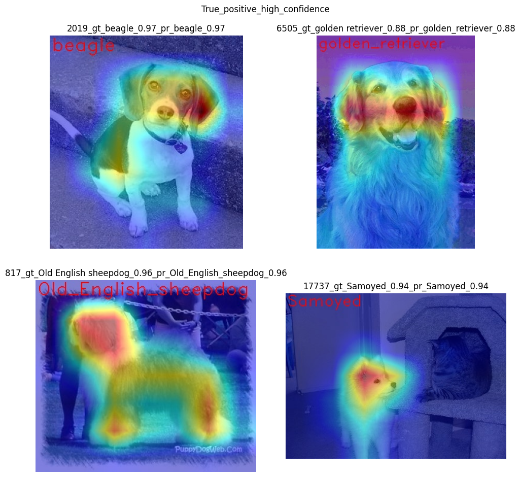
In the case of True positive high confidence, the model predicts the
correct class and is confident about its prediction.
The saliency map highlights features that strongly contribute to the correct class, meaning that those features are very salient for the current class. We want to roughly estimate that the highlighted features are correct. From the above images, we see that the dog’s face, nose, ears, and the general shape of the dog’s body usually contain the strongest features for the model. That correlates with our common knowledge and points to the fact that the model is well-trained and focuses on the needed areas.
Another sign that the model learns the right features is that the
classes are well distinguished by the model. Cat features are not used
at all to predict Samoyed in image 17737, which is the desired
behavior.
True Positive Low confidence#
show_use_case_image("True_positive_low_confidence")
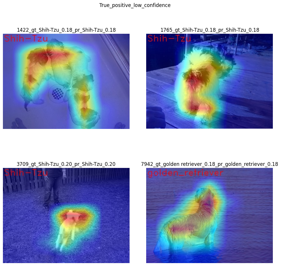
True positive low confidence basically means that key features are
not well available or are transformed. From the saliency maps, we see
that the model is paying attention to the whole object, trying to make a
decision mostly based on high-level features.
False Positive High confidence#
show_use_case_image("False_positive_high_confidence")
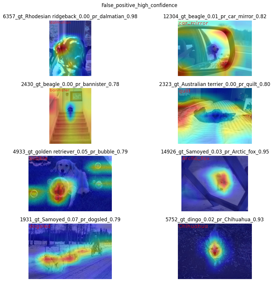
Here we see a few different reasons why the model can predict one class instead of another:
There are objects of two classes represented in the image, and one class is much more obvious than the other. For example, it’s larger or in the foreground. We can see this in the image
2430(bannisterinstead ofbeagle),1931(dogsledinstead ofsamoyed),2323(quiltinstead ofAustralian terrier),12304(car mirrorinstead ofbeagle).We can see that it’s not the problem of the model but rather the characteristic of the picture itself. In multiclass classification with only one annotated class in the image (and softmax applied to the model), this can happen if features of the wrong class dominate the features of the right class. Also, this might indicate a labeling error.
Two classes look similar in specific shooting settings.
In the picture
5752, the bigdingodog was confused with a smallchihuahua, focusing only on the face features. In the picture14926, a sleepingsamoyedwas confused with anarctic foxbecause the sleeping position distorted the key features, making the classes look even more alike than usual. In the picture6357, shadows created a pattern on the dog, so the model found key features for thedalmatianclass and predicted it with high confidence.
As a result, we see that the model is well-trained and mixes classes only because of intricate shooting conditions and the presence of more than one class in the picture.
Two mixed predictions#
show_use_case_image("True_positive_two_predictions")
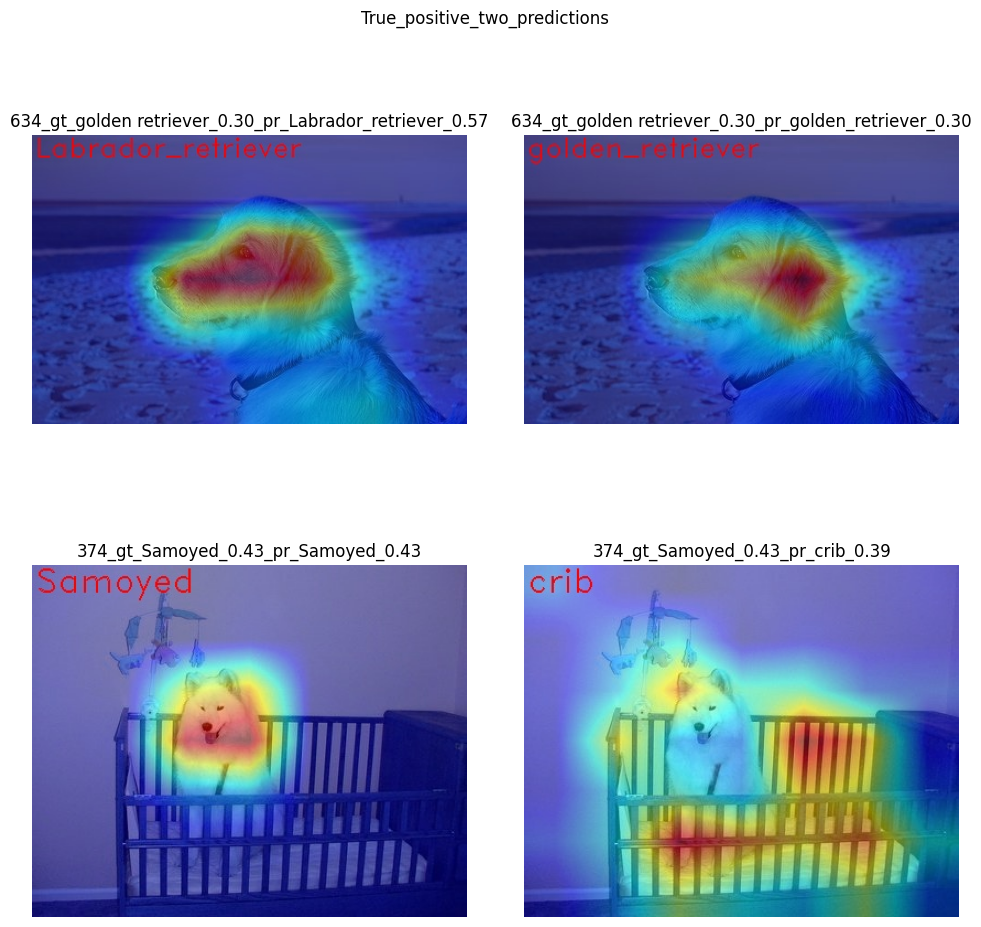
Here are examples where two classes are predicted with relatively high confidence, and the model is sure about both of them. We can see how saliency maps are different for each class.
In the picture 634, the model can’t decide between
golden retriever and labrador, focusing on the whole face shape.
In the image 374, both samoyed and crib are well-seen, so
the model cannot decide between these two classes. We clearly see the
different areas of interest for each of these classes.