View Inference Results
Inference Results
Once an initial inference has been run with your project, you can view performance results on the Analyze tab of the Projects page.
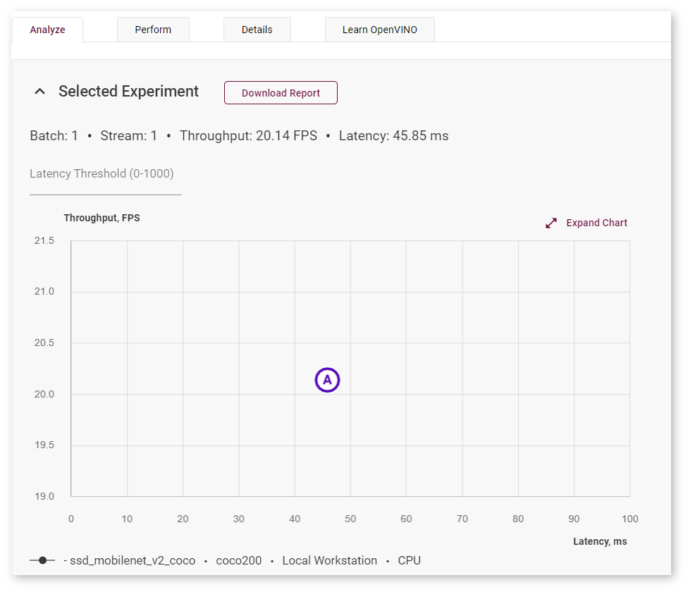
Throughput/Latency graph
Table with inferences
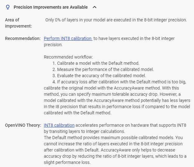
If there are ways to improve the performance of your model, the DL Workbench notifies you in the Analyze tab:
Clicking this button taken you to the bottom of the page with the detailed information on what can be improved and what steps you should take to get the most possible performance of this project.
Scroll down to the three tabs below:
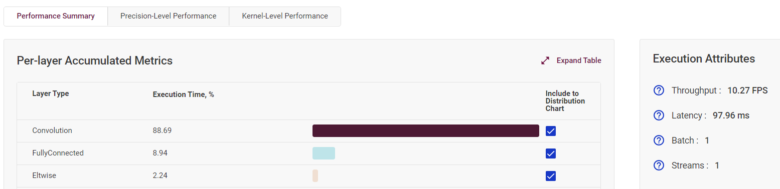
Performance Summary Tab
The tab contains the Per-layer Accumulated Metrics table and the Execution Attributes field, which includes throughput, latency, batch, and streams values of the selected inference.
Click Expand Table to see the full Per-layer Accumulated Metrics table, which provides information on execution time of each layer type as well as the number layers in a certain precision. Layer types are arranged from the most to the least time taken.
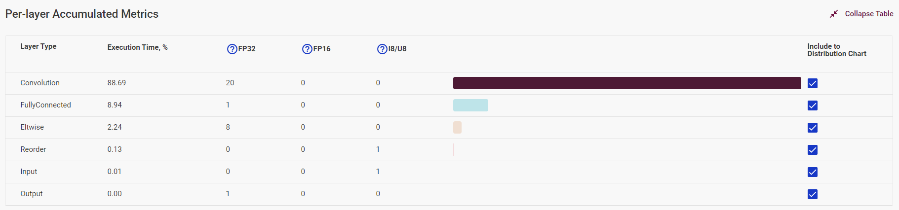
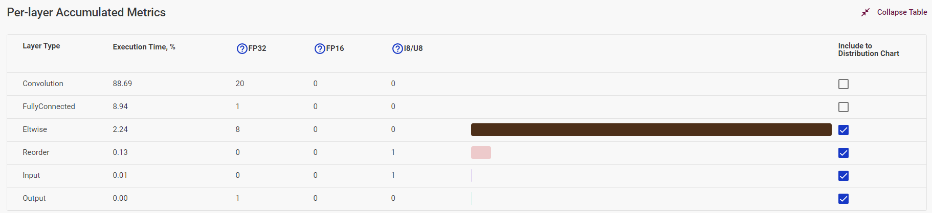
The table visually demonstrates the ratio of time taken by each layer type. Uncheck boxes in the Include to Distribution Chart column to filter out certain layers.
Precision-Level Performance Tab
The tab contains the Precision Distribution table, Precision Transitions Matrix, and Execution Attributes.
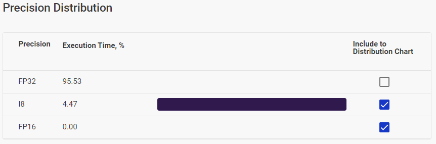
The Precision Distribution table provides information on execution time of layers in different precisions.
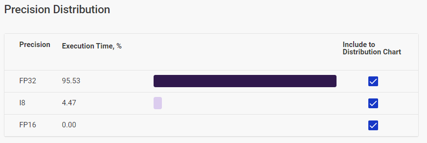
The table visually demonstrates the ratio of time taken by each layer type. Uncheck boxes in the Include to Distribution Chart column to filter out certain layers.
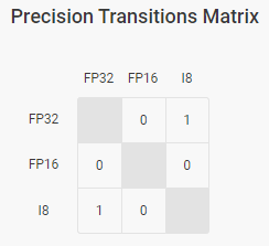
The Precision Transitions Matrix shows how inference precision changed during model execution. For example, if the cell at the FP32 row and the FP16 column shows 8, this means that eight times there was a pattern of an FP32 layer being followed by an FP16 layer.
Kernel-Level Performance Tab
The Kernel-Level Performance tab includes the Layers table and model graphs. See Visualize Model for details.
The Layers table shows each layer of the executed graph of a model:
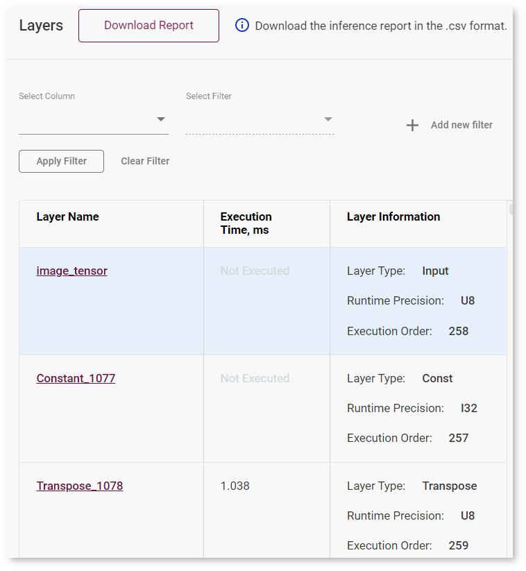
For each layer, the table displays the following parameters:
Layer name
Execution time
Layer type
Runtime precision
Execution order
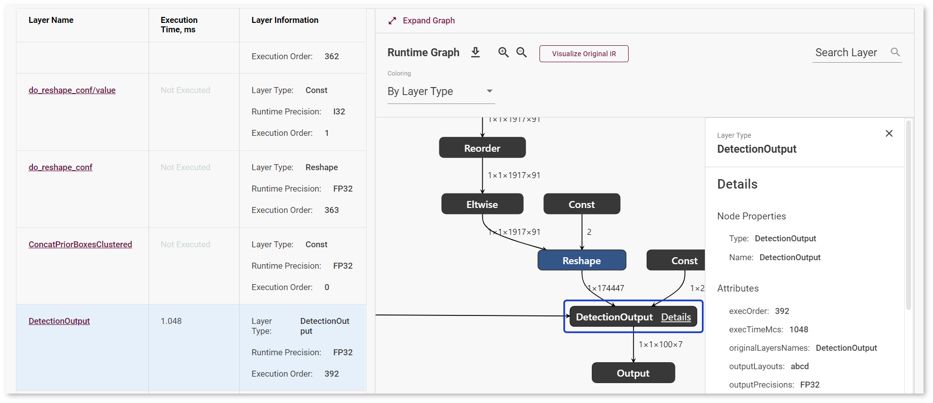
To see details about a layer:
Click the name of a layer. The layer gets highlighted on the Runtime Graph on the right.
Click Details next to the layer name on the Runtime Graph. The details appear on the right to the table and provide information about execution parameters, layer parameters, and fusing information in case the layer was fused in the runtime.
Tip
To download a .csv inference report for your model, click Download Report.
Sort and Filter Layers
You can sort layers by layer name, execution time, and execution order (layer information) by clicking the name of the corresponding column.
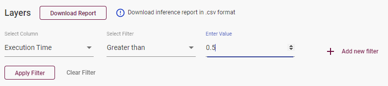
To filter layers, select a column and a filter in the boxes above the table. Some filters by the Execution Order and Execution Time columns require providing a numerical value in the box that is opened automatically:
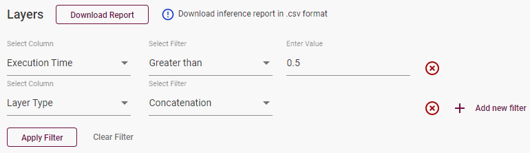
To filter by multiple columns, click Add new filter after you specify all the data for the the current column. To remove a filter, click the red remove symbol on the left to it:
Note
The filters you select are applied simultaneously.
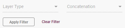
Once you configure the filters, press Apply Filter. To apply a different filter, press Clear Filter and configure new filters.
Per-Layer Comparison
To compare layers of a model before and after calibration, follow the steps described in Compare Performance between Two Versions of Models. After that, find the Model Performance Summary at the bottom of the page.
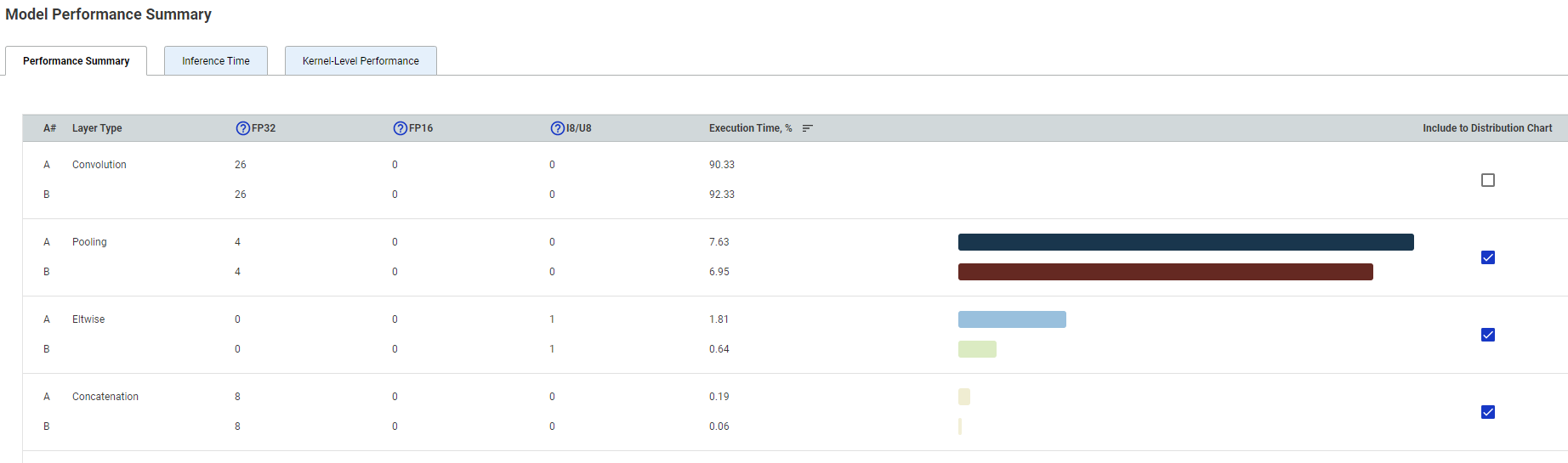
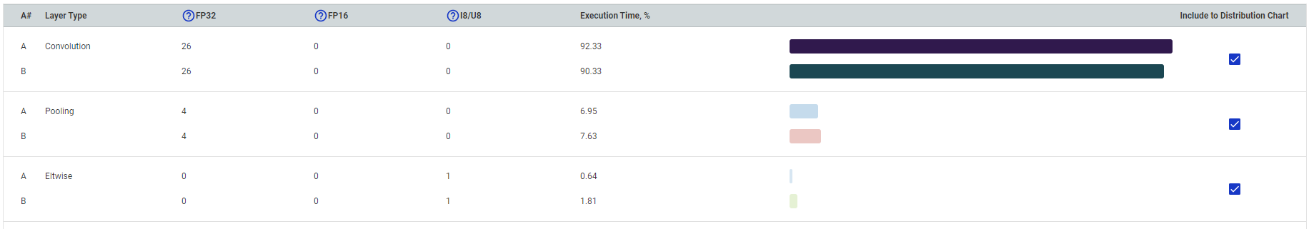
The Performance Summary tab contains the table with information on layer types of both projects, their execution time, and the number of layers of each type executed in a certain precision.
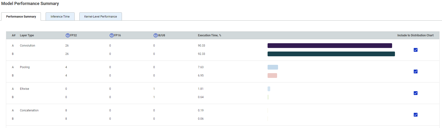
You can sort values in each column by clicking the column name. By default, layer types are arranged from the most to the least time taken. The table visually demonstrates the ratio of time taken by each layer type. Uncheck boxes in the Include to Distribution Chart column to filter out certain layers.
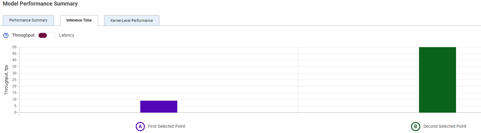
The Inference Time tab compares throughput and latency values. By default, the chart shows throughput values. Switch to Latency to see the difference in latency values.
The Kernel-Level Performance tab
Note
Make sure you select points on both graphs.
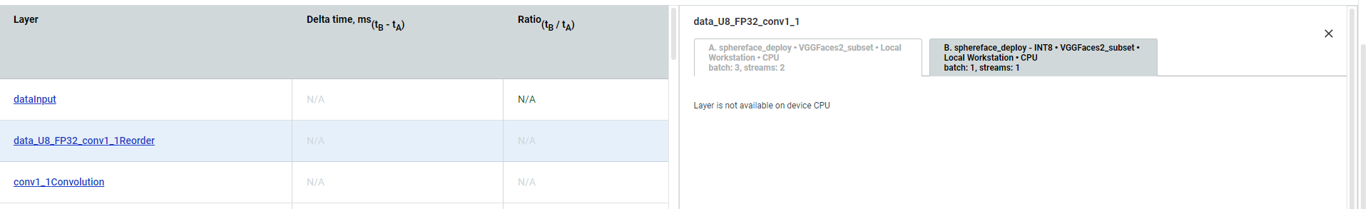
Each row of a table represents a layer of executed graphs of different model versions. The table displays execution time and runtime precision. If a layer was executed in both versions, the table shows the difference between the execution time values of different model versions layers.
Click the layer name to see the details that appear on the right to the table. Switch between tabs to see parameters of layers that differ between the versions of the model:
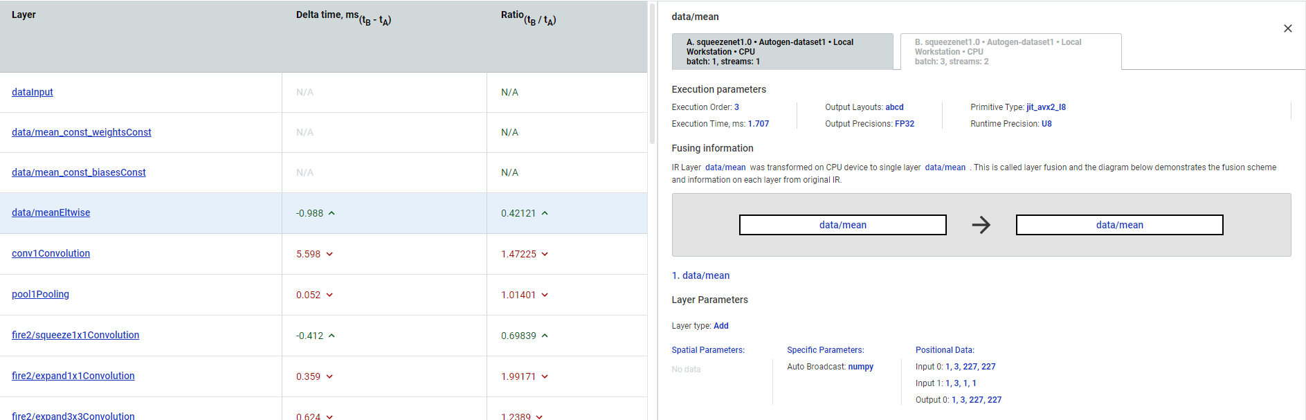
In case a layer was not executed in one of the versions, the tool notifies you: