After you have run an initial inference, and your performance data is visible on the dashboard, you can evaluate performance and tune your model. The data appears in the Model Performance Summary on the Projects page. When you have multiple inference results, you can click on specific data points to view model performance details.
The Layers Table at the bottom of the page shows each layer of the executed graph of a model: 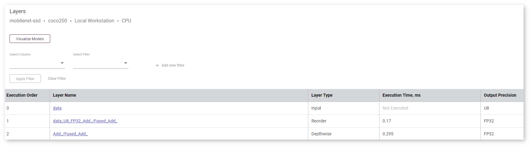
For each layer, the table displays the following parameters:
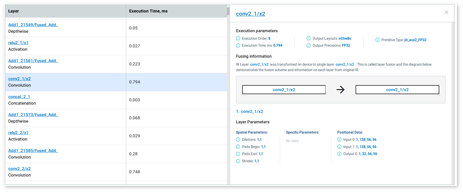
To see details about a layer, click its name. The details appear on the right to the table and provide information about execution parameters, layer parameters, and fusing information in case the layer was fused in the runtime.
You can sort the table by any parameter by clicking the name of the corresponding column.
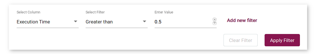
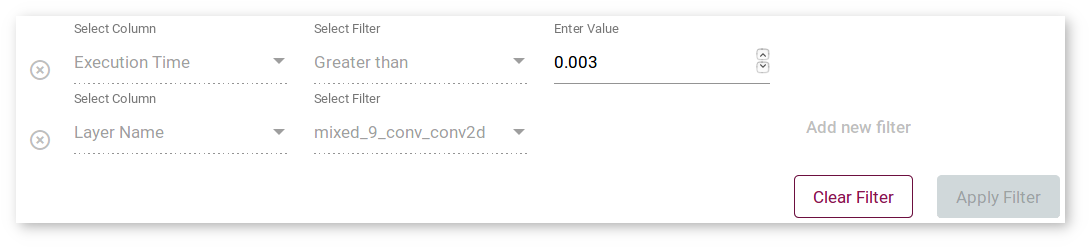
To filter layers, select a column and a filter in the boxes above the table. Some filters by the Execution Order and Execution Time columns require providing a numerical value in the box that is opened automatically:
To filter by multiple columns, click Add new filter after you specify all the data for the the current column. To remove a filter, click the red remove symbol on the left to it:
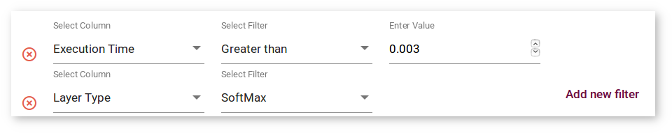
NOTE: The filters you select are applied simultaneously.
To apply a different filter, click the Clear Filter button and correct the previous parameters.
To compare layers of a model before and after calibration, follow the steps described in Compare Performance between Two Versions of Models. After that, find the Layers Table at the bottom of the page:
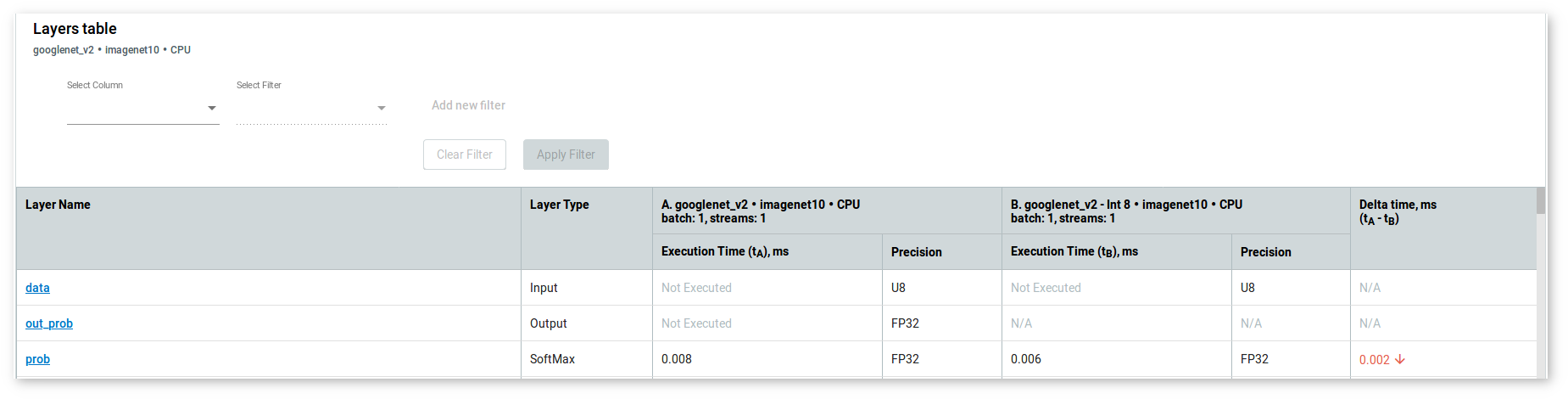
NOTE: Make sure you select points on both graphs.
Each row of a table represents a layer of executed graphs of different model versions. The table displays execution time and precision. If a layer was executed in both versions, the table shows the difference between the execution time values of different model versions layers .
Click the layer name to see the details that appear on the right to the table. Switch between tabs to see parameters of layers that differ between the versions of the model: 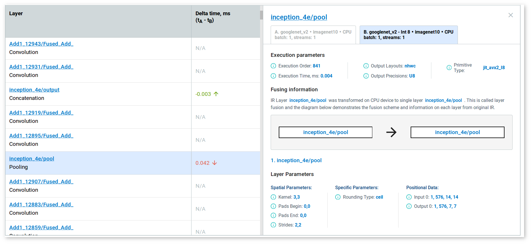
In case a layer was not executed in one of the versions, the tool notifies you: 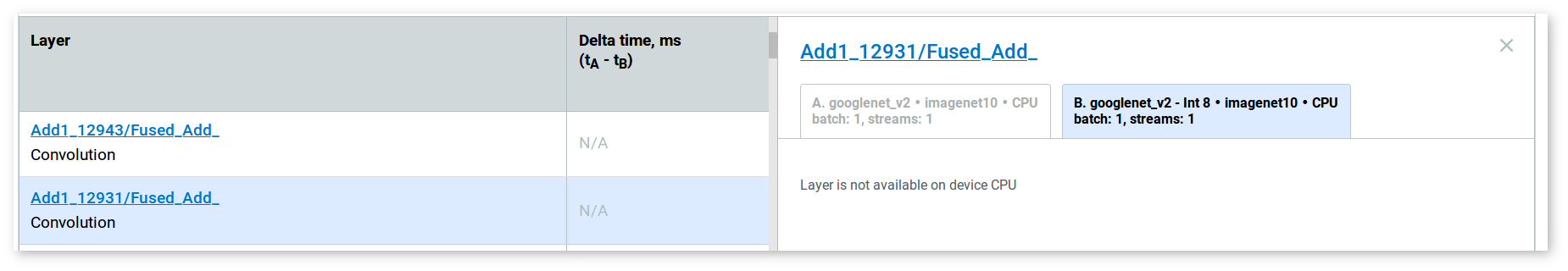
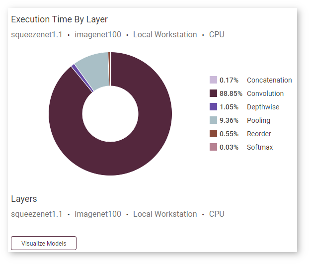
Use the Visualize Models button under the Execution Time by Layer donut chart to visualize your model:
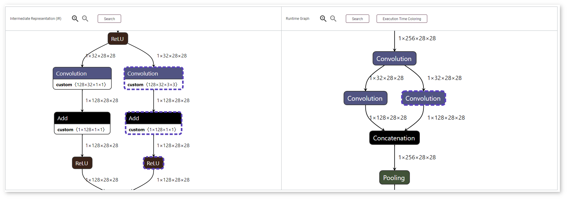
The panel with two graphs opens below. The graph on the right shows an original model in the OpenVINO™ IR format before it is executed by the Inference Engine, and the graph on the right shows how a model looks when it is executed by the Inference Engine.
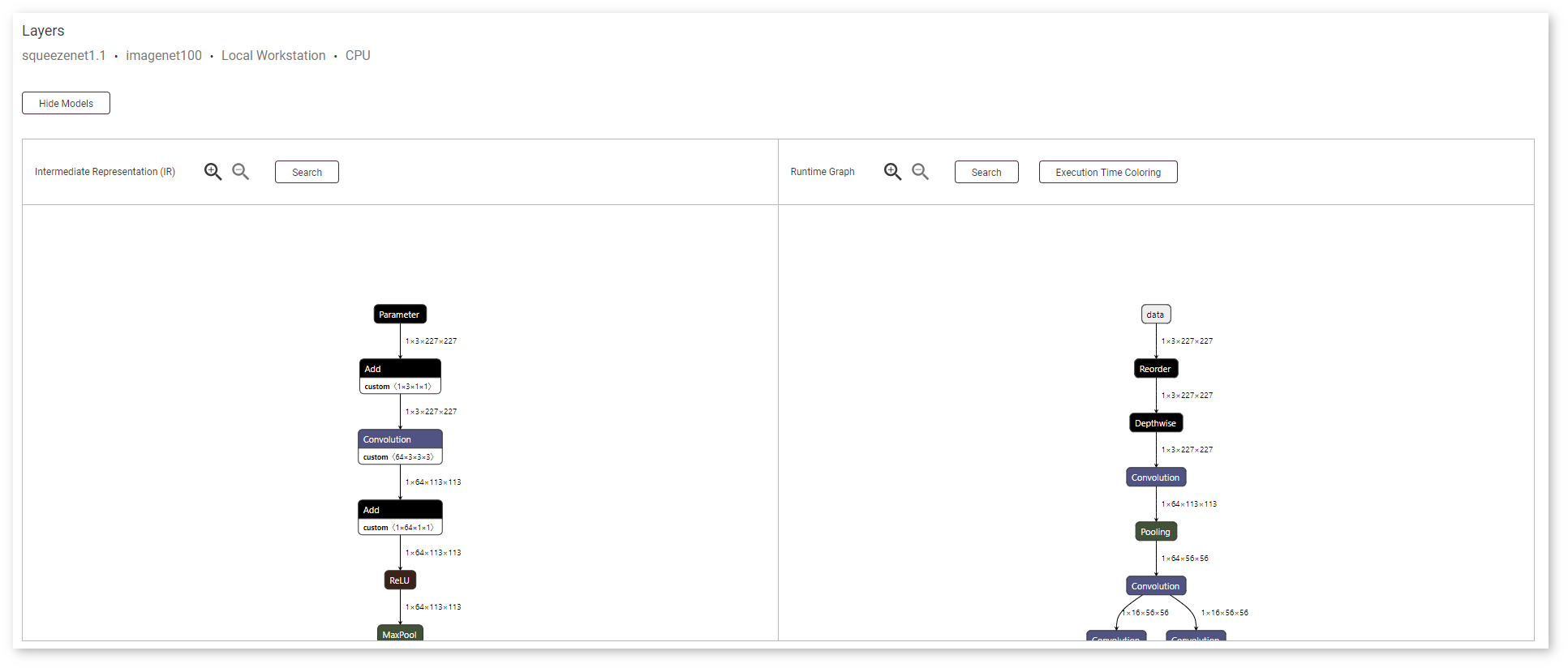
Layers in the runtime graph and the IR (Intermediate Representation) graph have different meanings. The IR graph reflects the structure of a model, while the runtime graph shows how a specific version of the model was executed on a specific device. The runtime graphs usually have different structures for different model versions and for the same model run on different devices, because every device executes models in a certain way to achieve the best performance.
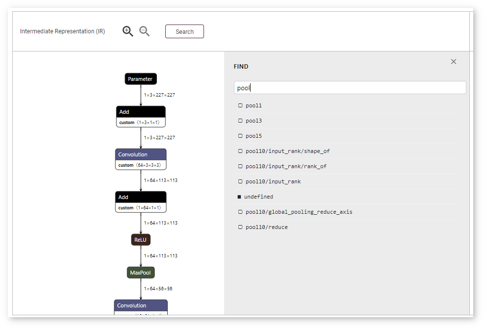
To adjust the scale, use magnifying glass icons or your mouse scroll wheel. To quickly find a layer, use the Search button. Enter a layer name or input dimensions in the FIND field that opens:
To learn details about a layer, click its name. The Node Properties window appears on the right: 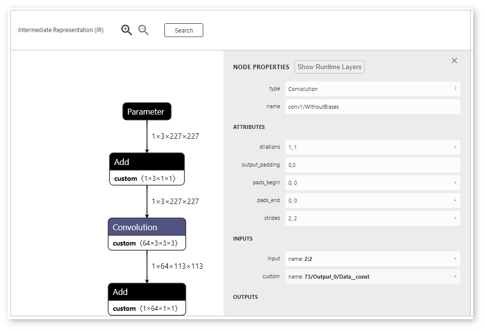
DL Workbench supports mapping between runtime and execution layers, which visually represents whether a layer was fused, tiled, or stayed intact. Use the Show Runtime Layers and Show Original Layers buttons correspondingly. Analogous layers are highlighted with dashed borders.
If a layer does not have a corresponding layer, the button is disabled: 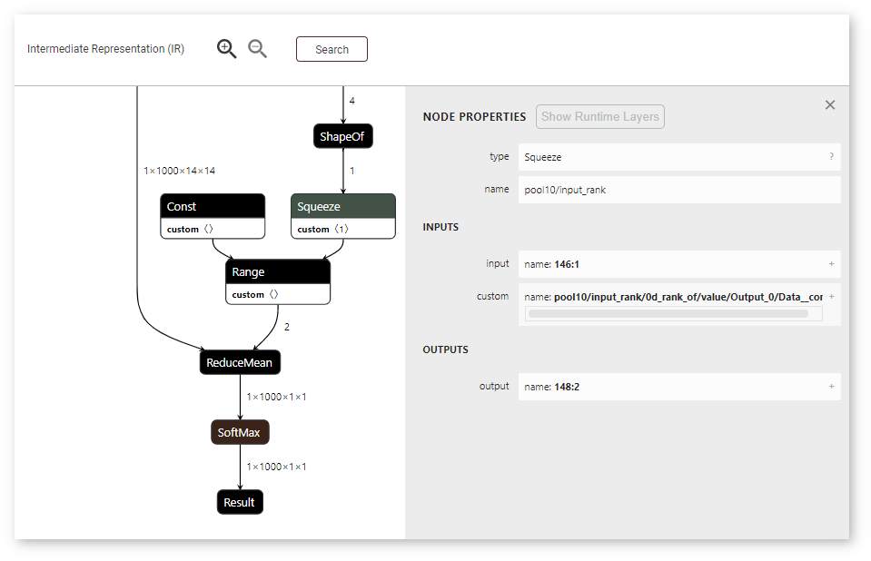
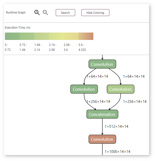
You can also visualize execution time of layers. Click Execution Time Coloring on the Runtime Graph side. The graph gets colored according to the scale that appears above it. To return to the generic view, click Hide Coloring.
To learn about graph optimization algorithms supported on different plugins, see the Inference Engine CPU, Intel® Processor Graphics, and Intel® Movidius™ Neural Compute Stick 2 and Intel® Vision Accelerator Design with Intel® Movidius™ VPUs supported plugins documentation. For additional details on reading graphs of a model executed on a VPU plugin, see the section below.
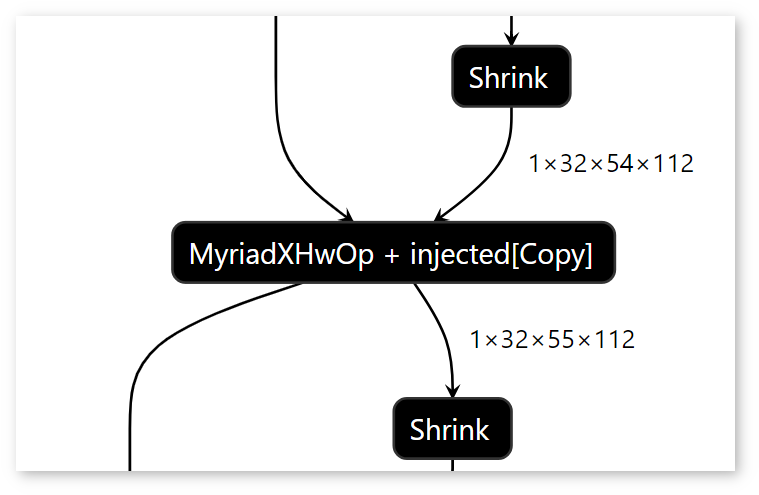
If layers are joined, the Runtime graph displays an HwOp layer with two input and two output layers:
In the Runtime graph, FullyConnected, GEMM, and 3D Convolution layers are expressed as a sequence of 2D Convolution layers.
Certain graph features may be the signs of a low-performance model:
NOTE: Intel® Neural Compute Stick 2 does not support asymmetrical paddings. Therefore, asymmetrical paddings in the Intermediate Representation (IR) graph result in several Pad layers in the Runtime Graph, which causes lower performance of a model.
